Preparing data without leakage

Mastering AI · Technical phase · Week 1 · Part 14

Goal of this step

In part 13, we split the data at random, and that was fine: the points were independent. On time-ordered traces, the very same move produces scores that are too good to be true.

By the end of this article you’ll be able to:

• generate a first set of simulated memory traces, with features and labels;
• recognize the three big families of data leakage;
• split time-ordered data correctly: time-based split with purge;
• measure, with numbers, how much a leak inflates a score.

---

Key concepts

1. Train, validation, test: three different roles

Intuition. The test set is a surprise exam. If the student has seen the questions, even indirectly, the grade means nothing.

Set	Used to	Rule
Train	fit the parameters $\theta$	the model sees it as much as it wants
Validation	choose hyperparameters, features, the model	we look at it often, so it ends up slightly “learned”
Test	estimate final performance	we look at it only once, at the end

The estimate of the true risk from part 13 is only valid if no information from the test set has influenced the model. That’s exactly the condition leaks violate.

2. The three families of leakage

Intuition. A leak is when the model gets, during training, a piece of information it will never have in production.

1. Leak from the future. A feature computed with values from after the prediction time. Typical example: a centered rolling mean (looking 5 steps back and 5 steps ahead).
2. Leak through the split. Nearly identical examples end up on both sides of the split. In a time series, time $t$ and time $t+1$ of the same region look extremely alike. If one is in train and the other in test, the model “recognizes” the answer instead of predicting it.
3. Leak through preprocessing. We scale, impute or select features on all the data before splitting. Test-set statistics then flow into training. The effect is often small, but real, and it gets strong with feature selection.

The rule that covers all three: anything that learns something from the data (model, scaler, imputer, selector) is fitted on the train set only. In practice, we wrap these steps in a scikit-learn Pipeline, which guarantees that fit only sees the train set.

3. The time-based split, and why it needs a purge

Intuition. In production, we train on the past and predict the future. The evaluation must reproduce exactly that situation.

We cut at a time $t_c$ : everything before is for training, everything after is for testing.

Subtlety: our label looks at the future. $y_t = 1$ if the region is accessed between $t+1$ and $t+H$ . A training example just before $t_c$ therefore has a label that depends on what happens after $t_c$ , i.e. in the test period. We remove those examples: that’s the purge.

$$\text{train} = \{\, t < t_c - H \,\} \qquad \text{test} = \{\, t \ge t_c \,\}$$

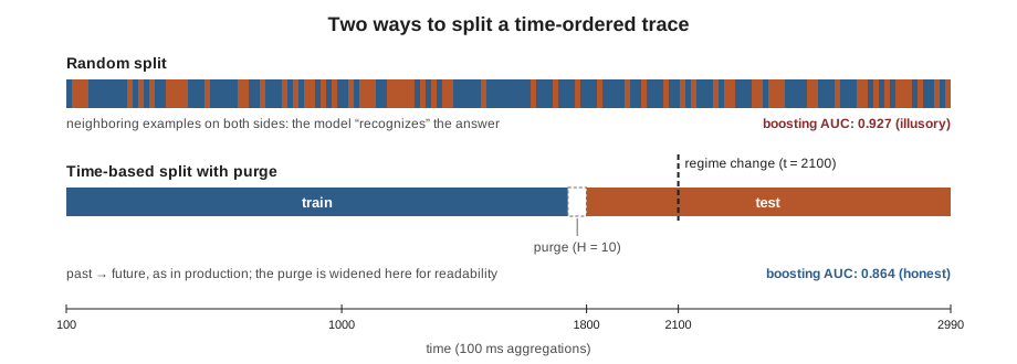
The two AUCs in the figure are the ones we get further down in the code example.

4. Sliding-window features

Intuition. To decide whether a region will be read again, we summarize its recent past in a few numbers: how many accesses, since when, at what pace.

For one region, at each aggregation $t$ , using only $a_{t-k}, \dots, a_t$ :

Feature	What it captures
mean_5, mean_20, mean_100	access intensity at several time scales
frac_active_20	regularity: share of the last 20 aggregations with at least one access
since_last	recency: the information LRU uses
est_period	gap between the last two activity starts
phase	since_last / est_period: where are we in the cycle?
neighbors_mean_5	activity of adjacent regions (locality)

est_period and phase are a simple version of the “periodicity” in your hypothesis H1. The rigorous version goes through autocorrelation → Required Maths M7: variance, covariance.

---

Code example

The full script does four things: simulate the traces, build the dataset, compare random and time-based splits, then show two classic leaks. The four blocks below go one after the other in the same file; the whole thing runs in about ten seconds (numpy 2.5, pandas 3.0, scikit-learn 1.9).

Simulating the traces

We simulate 96 regions over 3,000 aggregations of 100 ms, i.e. 5 minutes. Regions come in blocks of 4 neighbors of the same kind, to mimic memory locality. There are four behaviors:

• periodic: a few active aggregations every 15 to 60 (think JVM GC cycles);
• hot: accessed almost all the time;
• cold: almost never accessed;
• bursty: random on/off periods.

At 70% of the trace, about 40% of the blocks draw a new behavior (which may land on the old one). That’s a workload regime change, as in real life.

import numpy as np
import pandas as pd
from sklearn.model_selection import train_test_split
from sklearn.pipeline import make_pipeline
from sklearn.preprocessing import StandardScaler
from sklearn.linear_model import LogisticRegression
from sklearn.ensemble import HistGradientBoostingClassifier
from sklearn.metrics import roc_auc_score

rng = np.random.default_rng(7)

T = 3000          # number of aggregations (100 ms each -> 5 minutes)
N_REGIONS = 96    # memory regions
BLOCK_SIZE = 4    # neighboring regions of the same kind (locality)
H = 10            # horizon: 10 aggregations = 1 s
T_CHANGE = int(0.7 * T)  # workload regime change

KINDS = ["periodic", "hot", "cold", "bursty"]


def simulate_segment(kind, length, rng):
    """Number of accesses per aggregation for one region of a given kind."""
    t = np.arange(length)
    if kind == "periodic":
        period = rng.integers(15, 60)
        duration = rng.integers(2, 5)
        phase = rng.integers(0, period)
        active = ((t + phase) % period) < duration
        return active * rng.poisson(6, length)
    if kind == "hot":
        return rng.poisson(rng.uniform(1.0, 4.0), length)
    if kind == "cold":
        return rng.poisson(0.01, length)
    # bursty: random on/off alternation (Markov chain)
    accesses = np.zeros(length, dtype=int)
    on = False
    for i in range(length):
        if not on and rng.random() < 0.02:
            on = True
        elif on and rng.random() < 0.15:
            on = False
        accesses[i] = rng.poisson(5) if on else 0
    return accesses


def simulate_traces(rng):
    """(regions x time) matrix; some regions change kind at T_CHANGE."""
    accesses = np.zeros((N_REGIONS, T), dtype=int)
    for block in range(N_REGIONS // BLOCK_SIZE):
        before = rng.choice(KINDS, p=[0.35, 0.2, 0.25, 0.2])
        after = rng.choice(KINDS) if rng.random() < 0.4 else before
        for r in range(block * BLOCK_SIZE, (block + 1) * BLOCK_SIZE):
            accesses[r, :T_CHANGE] = simulate_segment(before, T_CHANGE, rng)
            accesses[r, T_CHANGE:] = simulate_segment(after, T - T_CHANGE, rng)
    return accesses

Features and labels, without looking at the future

All pandas rolling windows are causal by default: the value at $t$ only uses $t$ and the past. The label, on the other hand, is deliberately computed on the future, and that’s the only place where the future is allowed to appear.

def region_features(a):
    """Features of one region, computed from the past only (t included)."""
    s = pd.Series(a, dtype=float)
    active = (a > 0).astype(float)
    f = pd.DataFrame({
        "accesses_t": s,
        "mean_5": s.rolling(5, min_periods=1).mean(),
        "mean_20": s.rolling(20, min_periods=1).mean(),
        "mean_100": s.rolling(100, min_periods=1).mean(),
        "frac_active_20": pd.Series(active).rolling(20, min_periods=1).mean(),
    })
    # time since last access, and estimated period between two activity starts
    since, period = np.empty(len(a)), np.empty(len(a))
    last, start, prev_start = -10**6, -10**6, -10**6
    for t in range(len(a)):
        if a[t] > 0:
            if t - last > 1:             # start of a new burst of activity
                prev_start, start = start, t
            last = t
        since[t] = min(t - last, 500)
        period[t] = min(start - prev_start, 500)
    f["since_last"] = since
    f["est_period"] = period
    f["phase"] = np.clip(since / np.maximum(period, 1), 0, 5)
    return f


def region_label(a, h=H):
    """y_t = 1 if the region is accessed within the next h aggregations."""
    active = (a > 0).astype(int)
    future = pd.Series(active[::-1]).rolling(h, min_periods=1).max().to_numpy()[::-1]
    y = np.zeros(len(a), dtype=int)
    y[:-1] = future[1:]         # window t+1 .. t+h
    return y


def build_dataset(accesses):
    pieces = []
    for r in range(N_REGIONS):
        f = region_features(accesses[r])
        # activity of the immediate neighbors (regions r-1 and r+1) over the last 5 aggregations
        neighbors = [v for v in (r - 1, r + 1) if 0 <= v < N_REGIONS]
        f["neighbors_mean_5"] = np.mean(
            [pd.Series(accesses[v], dtype=float).rolling(5, min_periods=1).mean() for v in neighbors],
            axis=0)
        f["region"] = r
        f["t"] = np.arange(T)
        f["y"] = region_label(accesses[r])
        pieces.append(f)
    df = pd.concat(pieces, ignore_index=True)
    # drop the warm-up (incomplete history) and the end (incomplete label)
    return df[(df.t >= 100) & (df.t < T - H)].reset_index(drop=True)


accesses = simulate_traces(rng)
df = build_dataset(accesses)
FEATURES = ["accesses_t", "mean_5", "mean_20", "mean_100", "frac_active_20",
            "since_last", "est_period", "phase", "neighbors_mean_5"]
print(df.shape, "positive rate:", round(df.y.mean(), 3))

Output: (277440, 12) positive rate: 0.307. So we have 277,440 examples (one row per region and per aggregation), 30.7% of them positive.

Random split versus time-based split

The logistic regression’s scaler is inside the pipeline: it’s only fitted on the train set. Both splits use a test set of the same size, so the comparison is fair.

# --- Time-based split with purge ---
t_cut = int(0.6 * T)
train = df[df.t < t_cut - H]         # purge: train labels don't see the test period
test = df[df.t >= t_cut]

# --- Random split (the bad idea) ---
train_rand, test_rand = train_test_split(df, test_size=len(test) / len(df), random_state=0)


def evaluate(model, tr, te, features=FEATURES):
    model.fit(tr[features], tr.y)
    return roc_auc_score(te.y, model.predict_proba(te[features])[:, 1])


models = {
    "logistic": lambda: make_pipeline(StandardScaler(), LogisticRegression(max_iter=1000)),
    "boosting": lambda: HistGradientBoostingClassifier(max_iter=200, random_state=0),
}
for name, make in models.items():
    auc_rand = evaluate(make(), train_rand, test_rand)
    auc_time = evaluate(make(), train, test)
    print(f"{name:>10} | AUC random split: {auc_rand:.3f} | AUC time split: {auc_time:.3f}")

AUC is a score between 0.5 (chance) and 1 (perfect); we’ll cover it in detail in part 15. Results with seed 7:

Model	Random split	Time split
Logistic regression	0.799	0.793
Gradient boosting	0.927	0.864

Two lessons:

• the simple model barely moves. It has too little capacity to “recognize” neighboring examples, so the leak doesn’t help it;
• gradient boosting gains 6 AUC points thanks to the random split. That gain is entirely illusory. It comes from two things: nearly identical consecutive examples on both sides of the split, and the regime change that the random split lets the model “see” during training.

The more powerful the model, the more it exploits the leak. That’s why a bad protocol can make you believe an LSTM crushes LightGBM, or the reverse.

Two blatant leaks, as examples

# --- Blatant leak: a feature that looks at the future ---
df["centered_mean"] = df.groupby("region").accesses_t.transform(
    lambda s: s.rolling(11, center=True, min_periods=1).mean())
train = df[df.t < t_cut - H]
test = df[df.t >= t_cut]
auc_leak = evaluate(models["boosting"](), train, test, FEATURES + ["centered_mean"])
print(f"boosting + feature that sees the future: AUC = {auc_leak:.3f}")

# --- Leak through identifier + time ---
auc_id = evaluate(models["boosting"](), train_rand, test_rand, FEATURES + ["region", "t"])
print(f"boosting + region + t, random split: AUC = {auc_id:.3f}")

Leak	AUC
None (reference, time split)	0.864
Centered rolling mean	0.936
region + t as features, random split	0.951

• center=True: a single parameter is enough for the feature to see 5 aggregations into the future, which overlap precisely with the label window.
• region + t: with the random split, the model learns “region 42 around $t = 2500$ is hot” and recovers the answer by interpolation. These two columns mean nothing in production: region 42 of another process has nothing to do with it.

---

Running project: what this changes for the thesis

• Protocol. The time-based split with purge becomes the rule for every experiment. Your proposal already said so (“never random”); you now have the numbers that justify that choice, to cite in the Methodology chapter.
• Forbidden features. No region identifier, no raw address, no absolute timestamp. Only quantities relative to the region’s past.
• Regime change. The test period after $t_c$ contains a workload change. It’s a miniature version of your question Q3 (generalization), which we’ll handle properly in part 18 with leave-one-workload-out.
• Real DAMON traces will replace simulate_traces without changing anything else: that’s the whole point of separating simulation from dataset construction.

---

Hands-on exercise

1. Measure the purge. Replace train = df[df.t < t_cut - H] with train = df[df.t < t_cut] (no purge). Does the AUC move? Raise H to 50 and try again. Why does the effect grow with $H$ ?
2. Leak through preprocessing. Add a SelectKBest(f_classif, k=4) step (from sklearn.feature_selection) to the logistic pipeline. Then make a faulty version: select the 4 best features on the whole df, before the split. Compare the selected features and the AUCs.
3. No regime change. Set T_CHANGE = T (no change at all). Does the gap between random and time-based split shrink? What does that tell you about where the gap comes from?
4. New feature. Add max_50, the maximum number of accesses over the last 50 aggregations. Check that it only uses the past, then measure its effect on the boosting’s time-split AUC.
5. Running project. Take the problem statement you wrote in part 13 and complete it: list of retained features, time-based split with the purge size, and an explicit list of forbidden features.

Hint for question 1: the purge removes exactly $H$ aggregations per region. The longer the horizon, the more the labels at the end of the train set overlap the test period.

---

Further resources

• scikit-learn docs: Common pitfalls and recommended practices, section Data leakage.
• Kaufman et al., Leakage in Data Mining: Formulation, Detection, and Avoidance (KDD 2011): the reference on the taxonomy of leaks.
• Marcos López de Prado, Advances in Financial Machine Learning, chapter 7: purging and embargo for time series.
• Refresher: pandas: from raw data to a clean table, for rolling and groupby.

---

What you should be able to do before moving on

• Name the three families of leakage, with an example of each
• Spot a leak in a notebook: centered feature, preprocessing before the split, identifiers
• Implement a time-based split with purge and explain why the purge equals $H$
• Build strictly causal sliding-window features with pandas
• Wrap preprocessing in a scikit-learn Pipeline

Next part: Evaluating a classifier for real (part 15). Here we used AUC without discussing it; we’ll see why it isn’t enough when a false cold costs far more than a false hot, and how to choose the decision threshold.