October 19, 2026 · 14 min read

Evaluating a classifier for real

Confusion matrix, precision, recall, ROC and PR: picking the right metric and threshold when errors don't cost the same.

Mastering AI · Technical phase · Week 1 · Part 15

Goal of this step

In part 14, we judged models with AUC without discussing it. For the thesis, that isn’t enough: in the end, we have to decide, region by region, whether to compress it or not. And the two possible errors don’t cost the same at all. A region compressed and then read again right away (a false cold) stalls the application during decompression. A region kept in RAM when it’s no longer used (a false hot) wastes a bit of memory, nothing more.

By the end of this article you’ll be able to:

read a confusion matrix and derive precision, recall, F1 and the false-cold rate;
explain why accuracy misleads as soon as classes are imbalanced;
read a ROC curve and a precision-recall curve, and choose between them;
set the decision threshold from an asymmetric cost, on the validation set;
check whether a model’s probabilities are calibrated.

Key concepts

1. The confusion matrix

Intuition. For each region, there’s the truth (hot or cold) and the model’s decision. That makes four cells, and every metric is just a way of combining those four numbers.

We take “hot” as the positive class ( $y = 1$ : the region is accessed within the next $H$ aggregations).

	Predicted hot (keep)	Predicted cold (compress)
Actually hot	TP: true positive	FN: false cold (expensive)
Actually cold	FP: false hot (cheap)	TN: true negative

2. Precision, recall, F1, and the accuracy trap

Intuition. Precision answers “when the model says hot, is it right?”. Recall answers “among the truly hot regions, how many does it find?”.

\begin{aligned} \text{precision} &= \frac{TP}{TP + FP} \qquad \text{recall} = \frac{TP}{TP + FN} \\ F_1 &= \frac{2 \cdot \text{precision} \cdot \text{recall}}{\text{precision} + \text{recall}} \end{aligned}

$F_1$ is a harmonic mean: it collapses as soon as either one is bad.

Accuracy, the share of correct decisions, misleads as soon as classes are imbalanced. On our test set, 31% of regions are hot: a model that declares everything cold gets 68.9% accuracy… with zero recall. It would compress every hot region.

3. The false-cold rate

For zswap, the operational question is: among the regions we compress, how many get read again?

$\text{false-cold rate} = \frac{FN}{FN + TN} = P(\text{hot} \mid \text{declared cold})$

That’s exactly the probability computed with Bayes in Required Maths M8. It depends on the model and on the base rate of hot regions: the same model doesn’t have the same false-cold rate on another workload.

4. ROC and precision-recall curves

Intuition. A model doesn’t output a decision, it outputs a score $p \in [0, 1]$ . The decision comes from a threshold: hot if $p \ge s$ . Each threshold gives a different confusion matrix; a curve shows them all at once.

The ROC curve plots recall (true positive rate) against the false positive rate $FP / (FP + TN)$ . Chance gives the diagonal.
The ROC AUC has a simple probabilistic meaning: it’s the probability that a randomly drawn hot region has a higher score than a randomly drawn cold region. It’s an expectation over pairs, in the spirit of Required Maths M7; we check it by simulation below.
The precision-recall curve (PR) plots precision against recall. Chance gives a horizontal line at the height of the base rate (0.311 here). Its area is called average precision (AP).

Which one to pick? ROC doesn’t depend on the base rate: handy to compare models across workloads. PR shows what happens on the rare class: when positives are scarce, a flattering ROC can hide poor precision (Saito and Rehmsmeier, 2015).

5. Choosing the threshold with an asymmetric cost

Intuition. The 0.5 threshold is nothing special: it amounts to saying a false cold and a false hot cost the same. That’s not our case.

Let $c_{FN}$ be the cost of a false cold and $c_{FP}$ the cost of a false hot. For a region with probability $p$ of being hot:

compressing it costs $p \, c_{FN}$ on average;
keeping it costs $(1 - p) \, c_{FP}$ on average.

So we keep it when $(1 - p)\,c_{FP} < p\,c_{FN}$ , i.e.:

$p > s^\star = \frac{c_{FP}}{c_{FP} + c_{FN}}$

With $c_{FN} = 10$ and $c_{FP} = 1$ , we get $s^\star = 1/11 \approx 0.091$ . This ratio of 10 is a working assumption: measuring the real cost of a zswap decompression against the memory gain will be part of the thesis.

This calculation assumes $p$ is a true probability. Otherwise, we choose the threshold empirically, by minimizing the average cost on the validation set, never on the test set (part 14).

6. Calibration

Intuition. A model is calibrated if, among the regions it gives $p = 0.2$ , about 20% are actually hot. A good ranking (a good AUC) doesn’t guarantee good calibration.

We measure it in two ways:

a reliability diagram: group the predictions into bins of $p$ and compare the mean $p$ with the actual rate;
the Brier score, the mean squared error on the probabilities: $\frac{1}{n}\sum_i (p_i - y_i)^2$ .

Code example

We reuse the part 14 script as is (simulation, features, labels), then append the four blocks below in the same file. The time-based split now has three periods, each separated by a purge of $H$ :

train: $t < 1390$ ;
validation: $1400 \le t < 1790$ , to choose the threshold;
test: $t \ge 1800$ , looked at only once. It contains the regime change at $t = 2100$ .

Default threshold and confusion matrix

# Continues the part 14 script: df, FEATURES, H and T are already defined.
from sklearn.metrics import (confusion_matrix, precision_score, recall_score, f1_score,
                             accuracy_score, roc_auc_score, roc_curve,
                             precision_recall_curve, average_precision_score, brier_score_loss)

# --- Three periods, each purged by H: train | validation | test ---
t_val, t_test = 1400, 1800
train = df[df.t < t_val - H]
val = df[(df.t >= t_val) & (df.t < t_test - H)]
test = df[df.t >= t_test]

model = HistGradientBoostingClassifier(max_iter=200, random_state=0)
model.fit(train[FEATURES], train.y)
p_val = model.predict_proba(val[FEATURES])[:, 1]
p_test = model.predict_proba(test[FEATURES])[:, 1]
print(f"hot rate: val {val.y.mean():.3f} | test {test.y.mean():.3f}")


def false_cold_rate(y, pred):
    """Share of regions declared cold (hence compressed) that get read again: FN / (FN + TN)."""
    cold = pred == 0
    return (y[cold] == 1).mean()


def summary(y, p, threshold):
    pred = (p >= threshold).astype(int)
    tn, fp, fn, tp = confusion_matrix(y, pred).ravel()
    return dict(threshold=threshold, TP=tp, FP=fp, FN=fn, TN=tn,
                accuracy=accuracy_score(y, pred), precision=precision_score(y, pred),
                recall=recall_score(y, pred), f1=f1_score(y, pred),
                false_colds=false_cold_rate(y.to_numpy(), pred))


# 1. The default threshold, and the accuracy trap
r = summary(test.y, p_test, 0.5)
print(f"threshold 0.5: TP = {r['TP']}, FP = {r['FP']}, FN = {r['FN']}, TN = {r['TN']}")
print(f"accuracy {r['accuracy']:.3f} | precision {r['precision']:.3f} | recall {r['recall']:.3f} | "
      f"F1 {r['f1']:.3f} | false colds {r['false_colds']:.3f}")
print(f"\"everything is cold\": accuracy = {1 - test.y.mean():.3f}, recall = 0")

Threshold 0.5 on test	Value
TP / FP / FN / TN	24,305 / 4,149 / 11,274 / 74,512
Accuracy	0.865
Precision	0.854
Recall	0.683
$F_1$	0.759
False-cold rate	0.131
“Everything cold”: accuracy	0.689 (recall 0)

With the default threshold, the model looks good (86.5% accuracy, 85% precision). But 13.1% of compressed regions are read again within the next second: a third of the hot regions (11,274 out of 35,579) end up in zswap.

ROC, PR, and AUC as a probability

# 2. ROC and PR: curves that don't depend on any threshold
auc = roc_auc_score(test.y, p_test)
ap = average_precision_score(test.y, p_test)
rng_auc = np.random.default_rng(0)
i_pos = rng_auc.choice(np.flatnonzero(test.y == 1), 200_000)
i_neg = rng_auc.choice(np.flatnonzero(test.y == 0), 200_000)
p_wins = (p_test[i_pos] > p_test[i_neg]).mean() + 0.5 * (p_test[i_pos] == p_test[i_neg]).mean()
print(f"ROC AUC = {auc:.3f} | P(hot score > cold score) = {p_wins:.3f}")
print(f"average precision (PR AUC) = {ap:.3f} | chance = {test.y.mean():.3f}")

ROC AUC = 0.858, and the probability estimated on 200,000 (hot, cold) pairs is also 0.858: AUC is indeed $P(\text{score of a hot one} > \text{score of a cold one})$ .
Average precision = 0.828, versus 0.311 for chance.
AUC is a bit lower than in part 14 (0.864): training now stops at $t = 1390$ instead of 1790, to make room for validation.

The threshold that minimizes the cost

# 3. Choosing the threshold with an asymmetric cost (on validation, never on test)
C_FALSE_COLD, C_FALSE_HOT = 10, 1          # a false cold costs 10 times more


def average_cost(y, p, threshold):
    pred = p >= threshold
    fn = np.sum((y == 1) & ~pred)            # false colds: read again after being compressed
    fp = np.sum((y == 0) & pred)             # false hots: memory kept for nothing
    return (C_FALSE_COLD * fn + C_FALSE_HOT * fp) / len(y)


thresholds = np.linspace(0.01, 0.99, 99)
costs_val = [average_cost(val.y.to_numpy(), p_val, s) for s in thresholds]
s_val = thresholds[int(np.argmin(costs_val))]
s_theory = C_FALSE_HOT / (C_FALSE_HOT + C_FALSE_COLD)
print(f"optimal threshold on validation: {s_val:.2f} | theoretical threshold: {s_theory:.3f}")
for s in (0.5, s_val):
    r = summary(test.y, p_test, s)
    print(f"test, threshold {s:.2f}: cost = {average_cost(test.y.to_numpy(), p_test, s):.3f} | "
          f"precision {r['precision']:.3f} | recall {r['recall']:.3f} | "
          f"false colds {r['false_colds']:.3f} | compressed regions {(p_test < s).mean():.3f}")

Test	Threshold 0.5	Threshold 0.11 (chosen on validation)
Average cost per region	1.023	0.707
Precision	0.854	0.417
Recall	0.683	0.899
False-cold rate	0.131	0.096
Compressed regions	75.1%	32.9%

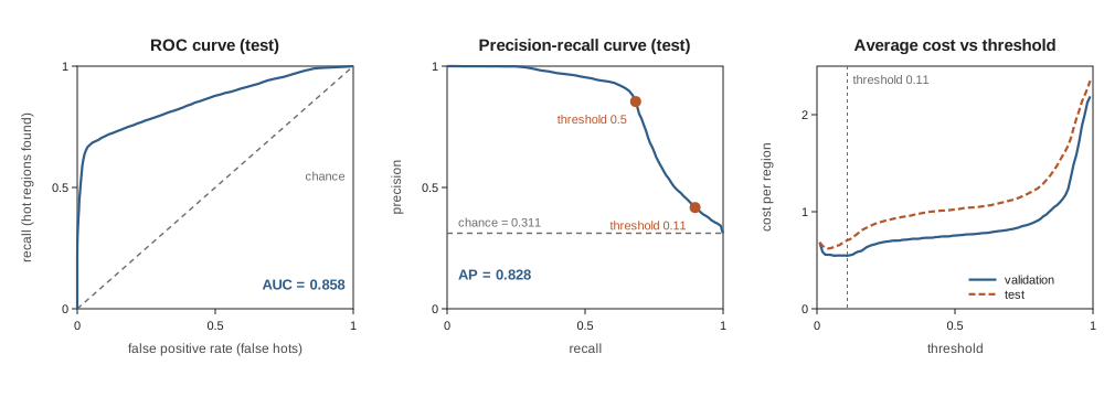
Four lessons:

the threshold found on validation (0.11) is close to the theoretical one (0.091): the model’s probabilities are roughly usable as they are;
lowering the threshold cuts the cost by 31%, but we compress far less (32.9% of regions instead of 75.1%). That’s the real trade-off of the thesis: memory gain versus false colds;
even at the best threshold, the false-cold rate stays at 9.6% on test. The orange curve in the figure shows why: after the regime change, the cost curve shifts, and the ideal test threshold is no longer the validation one. We don’t use it to choose (that would be a leak), but it’s a warning for production monitoring (part 28);
mind the right reference: never compressing costs $1 - 0.311 = 0.689$ per region on test, since every cold region becomes a false hot. At threshold 0.11, the model costs 0.707: slightly more than doing nothing. On validation, it clearly beat that reference (0.547 versus $1 - 0.301 = 0.699$ , see part 16); it’s the regime change that pushes it behind. So a model is compared first with “never compress”, not only with the 0.5 threshold.

Calibration

# 4. Calibration: does a probability of 0.2 mean "hot 1 time in 5"?
edges = [0, 0.05, 0.2, 0.4, 0.6, 0.8, 0.95, 1.0001]
for name, y, p in (("validation", val.y.to_numpy(), p_val), ("test", test.y.to_numpy(), p_test)):
    print(f"{name}: Brier = {brier_score_loss(y, p):.4f}")
    for a, b in zip(edges[:-1], edges[1:]):
        m = (p >= a) & (p < b)
        print(f"   p in [{a:.2f}, {min(b, 1):.2f}): n = {m.sum():>6} | mean p {p[m].mean():.3f} | "
              f"actual rate {y[m].mean():.3f}")

Bin of $p$	Mean $p$ (val)	Actual rate (val)	Mean $p$ (test)	Actual rate (test)
$[0, 0.05)$	0.020	0.021	0.024	0.043
$[0.05, 0.2)$	0.116	0.113	0.118	0.138
$[0.2, 0.4)$	0.275	0.146	0.274	0.170
$[0.4, 0.6)$	0.470	0.227	0.484	0.249
$[0.6, 0.8)$	0.716	0.688	0.713	0.602
$[0.8, 0.95)$	0.902	0.908	0.891	0.870
$[0.95, 1]$	0.987	0.994	0.990	0.982
Brier score	0.0827		0.1119

At the extremes, the model is well calibrated. In the 0.2 to 0.6 zone, it overestimates the probability of being hot: it announces 47%, reality is 23%. About 15% of validation regions (19% of test regions) fall there, but they are all above the chosen threshold (0.11): we keep them in RAM anyway, so this calibration error doesn’t change a single decision.
What matters for our threshold is the low zone. On validation, it’s very well calibrated (0.020 announced, 0.021 actual). On test, the actual rate doubles (0.024 announced, 0.043 actual): after the regime change, “surely cold” regions wake up. The Brier score goes from 0.083 to 0.112.

Running project: the protocol’s metrics

For the Methodology chapter of the thesis, each model (logistic regression, LightGBM, LSTM) will be reported with:

Metric	Why
ROC AUC	ranking quality, independent of the base rate, comparable across workloads
Average precision (AP)	quality on the hot class, sensitive to imbalance
Precision, recall, $F_1$ at the chosen threshold	readable by a jury
False-cold rate at the chosen threshold	the direct impact on latency with zswap
Share of compressed regions	the memory gain, the other side of the scale
Average cost, compared with “never compress”	does the model do better than doing nothing?
Brier and reliability diagram	are the probabilities usable for setting a threshold?

The threshold is always chosen on validation, with a cost ratio $c_{FN} / c_{FP}$ stated in advance, and the gaps between models are tested with the tools from Required Maths M9 (paired bootstrap, McNemar).

Hands-on exercise

False-cold rate under 1%. Find, on validation, the largest threshold that keeps the false-cold rate under 1%. What share of regions do we still compress? Apply that threshold to the test set: does the constraint hold? Explain with concept 3 and the calibration table.
Other costs. Redo the threshold choice with a $c_{FN} / c_{FP}$ ratio of 3, then 30. Each time, compare the threshold found on validation with the theoretical $s^\star$ .
Calibrate. Recalibrate the already trained model on validation: CalibratedClassifierCV(FrozenEstimator(model), method="isotonic").fit(val[FEATURES], val.y) (imports from sklearn.calibration and sklearn.frozen). Does the test Brier score improve? Does the optimal threshold move closer to $s^\star$ ?
The base-rate trap. Randomly subsample the hot regions of the test set so that they make up only 5% of the examples. At threshold 0.5, what happens to accuracy, precision, recall, ROC AUC and average precision? Which ones depend on the base rate, and which don’t?
Running project. Write the “Metrics” paragraph of the protocol in your notes: the seven metrics above, the chosen cost ratio and its justification, and the period on which the threshold is set.

Hint for question 1: on validation, a threshold around 0.03 is enough, and we then compress only about 15% of regions. Then look at the false-cold rate on test.

Further resources

scikit-learn docs: Metrics and scoring: quantifying the quality of predictions and Probability calibration.
Saito and Rehmsmeier, The Precision-Recall Plot Is More Informative than the ROC Plot When Evaluating Binary Classifiers on Imbalanced Datasets (PLOS ONE, 2015).
Fawcett, An introduction to ROC analysis (Pattern Recognition Letters, 2006).
Elkan, The Foundations of Cost-Sensitive Learning (IJCAI 2001): where the $c_{FP} / (c_{FP} + c_{FN})$ threshold comes from.

What you should be able to do before moving on

Read a confusion matrix and derive precision, recall, $F_1$ and the false-cold rate
Explain why accuracy misleads on imbalanced classes
Interpret ROC AUC as a probability, and choose between ROC and PR
Derive the optimal threshold $c_{FP} / (c_{FP} + c_{FN})$ and find it empirically on validation
Check a model’s calibration with a reliability diagram and the Brier score
Compare a model’s cost with that of “never compress”

Next part: Linear models and regularization (part 16). We open the box: the thesis’s logistic regression, its coefficients, and what the $L_1$ and $L_2$ penalties from M11 change in practice.