October 23, 2026 · 21 min read

Trees, forests and gradient boosting

Trees, bagging, boosting and LightGBM on the memory traces: how a tree finds on its own the bumps we built by hand, and the smallest model that keeps the gain.

Mastering AI · Technical phase · Week 2 · Part 17

Goal of this step

Since part 14, gradient boosting has won every table, and in part 16 we had to hand-build a “bump” feature so that logistic regression could see what boosting saw on its own. Time to open the box.

By the end of this article you’ll be able to:

explain how a decision tree picks a split (Gini impurity, entropy) and why its depth controls overfitting;
explain bagging versus boosting: averaging to reduce variance, or adding to reduce bias;
read gradient boosting as gradient descent in function space;
tune LightGBM’s main hyperparameters (num_leaves, n_estimators, learning_rate);
measure a model’s size and latency, and pick the smallest one that does the job.

Key concepts

1. A decision tree is a series of questions

Intuition. A tree asks “is phase ≤ 0.001?”, then, depending on the answer, another question, and so on. Each leaf holds a prediction: the share of hot regions among the training examples that ended up there.

To choose a question, the tree tries every feature and every threshold, and keeps the one that makes the two children as “pure” as possible. For a node with a fraction $p$ of positives, the Gini impurity is:

G(p) = 1 - p^2 - (1 - p)^2 = 2 p (1 - p)

It’s 0 for a pure node, maximal (0.5) at $p = 0.5$ . The gain of a split is the decrease of impurity, weighted by the size of each child:

\Delta G = G(p) - \frac{n_L}{n} G(p_L) - \frac{n_R}{n} G(p_R)

Entropy $H(p) = -p \log p - (1 - p) \log (1 - p)$ from Required Maths M8 plays the same role (the gain is then the information gain); in practice both choose almost the same splits.

Three properties follow directly:

a tree is invariant to monotonic transformations of a feature: since_last or log(since_last) give the same splits, so no need for a StandardScaler;
it builds non-monotonic effects by stacking two thresholds on the same feature: exactly what the linear model couldn’t do;
it’s greedy: each split is the best one now, without looking ahead.

2. Depth is capacity

Intuition. Each extra level doubles the number of leaves. With enough leaves, the tree can isolate each training example: it learns by heart.

A tree of depth $d$ has at most $2^d$ leaves. A shallow tree has high bias (it can’t express the real rule), a deep tree has high variance (it changes completely if you redraw the data). Depth, the minimum number of examples per leaf (min_samples_leaf) or the number of leaves are the knobs of the bias–variance trade-off from part 13.

3. Bagging and random forests: averaging to reduce variance

Intuition. A deep tree is unstable but not biased. Train several on slightly different data and average them: the errors partly cancel out.

Bagging (bootstrap aggregating) trains $B$ trees on bootstrap samples (draws with replacement) and averages their predictions. If each tree has variance $\sigma^2$ and two trees have correlation $\rho$ , the variance of the average is (Required Maths M7):

\operatorname{Var}\Big( \frac{1}{B} \sum_{b=1}^{B} f_b(x) \Big) = \rho \sigma^2 + \frac{1 - \rho}{B} \sigma^2

The second term vanishes when $B$ grows; the first stays. To reduce $\rho$ , the random forest only lets each split choose among a random subset of features (max_features="sqrt"): the trees disagree more, so their average is better.

4. Boosting: adding to reduce bias

Intuition. Instead of independent trees averaged together, we build small trees one after the other, each one fixing what the previous ones got wrong.

The model is a sum $F_M(x) = F_0 + \eta \sum_{m=1}^{M} h_m(x)$ , where $F$ is a score (a log-odds, as in part 16) and $\eta$ the learning rate. At each step, we compute the gradient of the log-loss with respect to each example’s score, and fit a small regression tree $h_m$ to minus that gradient:

r_i = - \frac{\partial \ell(y_i, F)}{\partial F} \bigg|_{F = F_{m-1}(x_i)} = y_i - \sigma\big(F_{m-1}(x_i)\big) \qquad F_m = F_{m-1} + \eta \, h_m

It’s exactly the gradient descent of Required Maths M10, except that we don’t move parameters $w$ : we move the function $F$ itself, one step = one tree. M10 did it by hand on the running project; here we use it to understand the hyperparameters:

n_estimators = number of steps, learning_rate = step size: halving one roughly requires doubling the other;
each tree is small (a few leaves): boosting starts from a high-bias model and reduces bias step by step. Too many steps and it overfits, hence early stopping on validation.

5. LightGBM: the same idea, fast

Intuition. Trying every threshold on 123,840 examples at every node is expensive. LightGBM first groups each feature’s values into at most 255 bins (histograms), then only tries the bin boundaries.

Two choices distinguish it:

leaf-wise growth: instead of filling a tree level by level, it always splits the leaf that reduces the loss the most. Size is controlled by num_leaves (number of leaves per tree), not by depth;
the main hyperparameters: num_leaves (complexity of each tree), n_estimators and learning_rate (number and size of steps), min_child_samples (minimum examples per leaf), max_depth (safety net, unlimited by default).

The HistGradientBoostingClassifier used since part 14 is scikit-learn’s reimplementation of these ideas (31 leaves, learning rate 0.1, 200 iterations in our settings).

6. Size and latency of a tree ensemble

Intuition. To predict, each tree walks from the root to a leaf: one comparison per level. The cost is proportional to the total number of trees times their depth, not to the number of training examples.

A tree with $L$ leaves has $L - 1$ internal nodes, i.e. $2L - 1$ nodes in total. An ensemble of $M$ trees therefore stores about $M (2L - 1)$ nodes. That’s the number to compare with the 12 weights of part 16’s logistic regression, and the one that will decide whether the model fits in a system daemon.

Code example

As in parts 15 and 16, we reuse the part 14 script as is (simulation, features, labels), then append the seven blocks below in the same file. Same split: train $t < 1390$ , validation $1400 \le t < 1790$ , test $t \ge 1800$ . The whole thing runs in about thirty seconds (numpy 2.5, pandas 3.0, scikit-learn 1.9, lightgbm 4.7).

How a tree chooses its first split

# Continues the part 14 script: df, FEATURES, H, np, pd and roc_auc_score are already defined.
import time
import lightgbm as lgb
from sklearn.tree import DecisionTreeClassifier, DecisionTreeRegressor
from sklearn.ensemble import RandomForestClassifier
from sklearn.linear_model import LogisticRegression
from sklearn.metrics import log_loss

# Same three periods as in parts 15 and 16
t_val, t_test = 1400, 1800
train = df[df.t < t_val - H]
val = df[(df.t >= t_val) & (df.t < t_test - H)]
test = df[df.t >= t_test]


# 1. How a tree chooses a split: Gini impurity, by hand
def gini(p):
    return 2 * p * (1 - p)        # impurity of a node with a fraction p of positives


def best_split(x, y):
    """Best threshold on one feature: largest weighted decrease of Gini impurity."""
    order = np.argsort(x, kind="stable")
    x, y = x[order], y[order]
    n = len(y)
    left_n = np.arange(1, n)                  # split after position i
    left_pos = np.cumsum(y)[:-1]
    right_n, right_pos = n - left_n, y.sum() - left_pos
    impurity = (left_n * gini(left_pos / left_n) + right_n * gini(right_pos / right_n)) / n
    valid = x[1:] != x[:-1]                    # only cut between two different values
    i = np.argmin(np.where(valid, impurity, np.inf))
    return (x[i] + x[i + 1]) / 2, gini(y.mean()) - impurity[i]


y_tr = train.y.to_numpy()
print(f"root impurity: {gini(y_tr.mean()):.4f}")
for f in FEATURES:
    s, gain = best_split(train[f].to_numpy(), y_tr)
    print(f"{f:>17} | threshold {s:8.3f} | Gini decrease {gain:.4f}")
stump = DecisionTreeClassifier(max_depth=1, random_state=0).fit(train[FEATURES], train.y)
print("scikit-learn root:", FEATURES[stump.tree_.feature[0]], round(stump.tree_.threshold[0], 3))

The root’s impurity is $G(0.307) = 0.4236$ .

Feature	Best threshold	Gini decrease
`accesses_t`	0.5	0.1027
`since_last`	0.5	0.1027
`phase`	0.001	0.1027
`frac_active_20`	0.475	0.0813
`mean_5`	0.3	0.0664
`mean_100`	0.625	0.0533
`mean_20`	2.225	0.0461
`neighbors_mean_5`	0.15	0.0275
`est_period`	36.5	0.0243

Three features tie exactly, and that’s no coincidence: accesses_t ≤ 0.5, since_last ≤ 0.5 and phase ≤ 0.001 all ask the same question, “was the region accessed at $t$ ?”. The first question a tree asks is LRU’s.
scikit-learn breaks ties through a random feature order: with random_state=0, it picks phase at 0.001. Our 15-line function finds the same threshold and the same gain.

The bump, found on its own

# 2. The bump that the linear model could not see, found by a tree on phase alone
grid = pd.DataFrame({"phase": [0.0, 0.25, 0.5, 0.75, 0.9, 1.0, 1.5, 3.0]})
lin = LogisticRegression().fit(train[["phase"]], train.y)
tree3 = DecisionTreeClassifier(max_depth=3, random_state=0).fit(train[["phase"]], train.y)
bump = lambda d: pd.DataFrame({"phase": d.phase, "near_cycle": np.exp(-((d.phase - 1) / 0.2) ** 2)})
lin_bump = LogisticRegression().fit(bump(train), train.y)       # part 16's hand-made bump
print(f"phase only | logistic AUC val {roc_auc_score(val.y, lin.predict_proba(val[['phase']])[:, 1]):.3f}"
      f" | logistic + near_cycle {roc_auc_score(val.y, lin_bump.predict_proba(bump(val))[:, 1]):.3f}"
      f" | depth-3 tree {roc_auc_score(val.y, tree3.predict_proba(val[['phase']])[:, 1]):.3f}")
print(pd.DataFrame({"phase": grid.phase,
                    "p logistic": lin.predict_proba(grid)[:, 1].round(3),
                    "p tree": tree3.predict_proba(grid)[:, 1].round(3)}).to_string(index=False))

`phase`	Logistic $p$	Depth-3 tree $p$
0	0.374	0.876
0.25	0.354	0.111
0.5	0.334	0.456
0.75	0.314	0.456
0.9	0.303	0.456
1.0	0.295	0.141
1.5	0.260	0.141
3.0	0.171	0.141

With phase alone, validation AUC goes from 0.670 (logistic) to 0.713 (logistic + part 16’s near_cycle bump) and to 0.803 (a depth-3 tree, i.e. 4 thresholds).

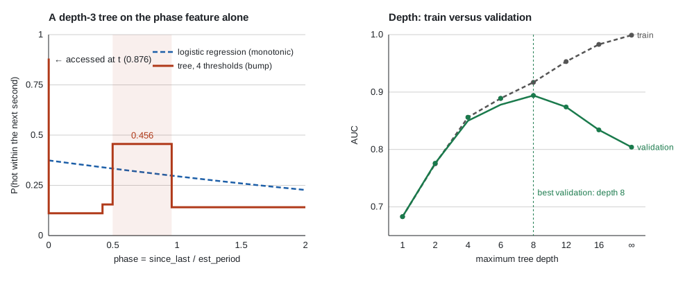
The tree uses its thresholds (0.001, 0.42, 0.499, 0.959) to draw a step function: very hot if accessed at $t$ , cold right after, a bump at 0.456 between 0.5 and 0.96, then cold again.
The bump isn’t where we put it by hand. In part 16, near_cycle was centered on 1. But the label looks 10 aggregations ahead: the next burst enters the window as soon as phase exceeds about $1 - H / \text{period}$ , i.e. between 0.33 and 0.83 for periods from 15 to 60. Beyond 1, the expected cycle didn’t come back: the region has probably left its periodic regime. The tree reads this from the data; we had guessed it, and slightly wrong.

Depth and overfitting

# 3. Depth = capacity: a tree that is too deep memorizes
for depth in [1, 2, 4, 6, 8, 12, 16, None]:
    t = DecisionTreeClassifier(max_depth=depth, random_state=0).fit(train[FEATURES], train.y)
    auc_tr = roc_auc_score(train.y, t.predict_proba(train[FEATURES])[:, 1])
    auc_va = roc_auc_score(val.y, t.predict_proba(val[FEATURES])[:, 1])
    print(f"depth {str(depth):>4} | {t.get_n_leaves():5d} leaves | AUC train {auc_tr:.3f} | AUC val {auc_va:.3f}")

Max depth	Leaves	Train AUC	Val AUC
1	2	0.683	0.683
2	4	0.775	0.776
4	16	0.856	0.850
6	58	0.889	0.878
8	186	0.917	0.894
12	1,013	0.953	0.874
16	2,658	0.983	0.834
unlimited	6,703	0.999	0.804

The textbook picture: up to depth 6 train and validation move together (bias goes down); beyond 8, train keeps rising towards 1 while validation drops (variance goes up). The unlimited tree knows the train set by heart (0.999) and does barely better than the logistic regression on validation (0.804 versus 0.808).

Bagging: five unstable trees, one stable average

# 4. Bagging: averaging unstable trees reduces variance
preds = []
for seed in range(5):
    boot = train.sample(frac=1.0, replace=True, random_state=seed)      # bootstrap sample
    t = DecisionTreeClassifier(max_features="sqrt", random_state=seed).fit(boot[FEATURES], boot.y)
    preds.append(t.predict_proba(val[FEATURES])[:, 1])
    print(f"deep tree {seed} | AUC val {roc_auc_score(val.y, preds[-1]):.3f}")
P = np.array(preds)
print(f"average of the 5 trees | AUC val {roc_auc_score(val.y, P.mean(axis=0)):.3f} | "
      f"mean correlation between trees {np.corrcoef(P)[np.triu_indices(5, 1)].mean():.2f}")
for n_trees in [1, 10, 100]:
    rf = RandomForestClassifier(n_estimators=n_trees, n_jobs=-1, random_state=0).fit(train[FEATURES], train.y)
    print(f"random forest, {n_trees:3d} trees | AUC val {roc_auc_score(val.y, rf.predict_proba(val[FEATURES])[:, 1]):.3f}")

Five deep trees, each trained on a bootstrap sample (with max_features="sqrt", as in a random forest, to decorrelate the trees), have a validation AUC between 0.810 and 0.820. Their average reaches 0.876: a gain of 6 points without any new information, only by averaging.
The predictions of two trees have a correlation of 0.70: that’s the $\rho$ in the formula, the part of the variance that averaging doesn’t remove.
The random forest goes from 0.802 (1 tree) to 0.887 (10 trees) and 0.899 (100 trees). Beyond that, it gains almost nothing: we’ve hit the $\rho \sigma^2$ floor.

Boosting by hand

# 5. Boosting = gradient descent in function space (M10), in 10 lines
X_tr, X_va = train[FEATURES].to_numpy(), val[FEATURES].to_numpy()
F_tr = np.full(len(y_tr), np.log(y_tr.mean() / (1 - y_tr.mean())))   # constant start: the base rate
F_va = np.full(len(X_va), F_tr[0])
for k in range(1, 51):
    residual = y_tr - 1 / (1 + np.exp(-F_tr))         # minus the log-loss gradient w.r.t. the score
    step = DecisionTreeRegressor(max_depth=3).fit(X_tr, residual)
    F_tr += 0.3 * step.predict(X_tr)                   # learning rate 0.3
    F_va += 0.3 * step.predict(X_va)
    if k in (1, 5, 20, 50):
        print(f"{k:2d} trees | log-loss train {log_loss(y_tr, 1 / (1 + np.exp(-F_tr))):.4f} | "
              f"AUC val {roc_auc_score(val.y, F_va):.3f}")

Trees	Train log-loss	Val AUC
1	0.5921	0.822
5	0.5274	0.826
20	0.4289	0.860
50	0.3768	0.865

Each tree has only 8 leaves (depth 3) and on its own would be weak. Their sum goes down the log-loss steadily: that’s descent, one tree per step. The line residual = y_tr - p is the whole idea: the log-loss gradient with respect to the score is $p - y$ (part 16), so the next tree learns what is still missing.

LightGBM: how many trees, how many leaves?

# 6. LightGBM: size, latency and cost, for several budgets
C_FALSE_COLD, C_FALSE_HOT = 10, 1


def average_cost(y, p, threshold):
    pred = p >= threshold
    return (C_FALSE_COLD * np.sum((y == 1) & ~pred) + C_FALSE_HOT * np.sum((y == 0) & pred)) / len(y)


thresholds = np.linspace(0.01, 0.99, 99)
y_va, y_te = val.y.to_numpy(), test.y.to_numpy()
X96 = test[test.t == t_test][FEATURES].to_numpy()      # the 96 regions at one aggregation
print(f"never compress | cost val {average_cost(y_va, np.ones(len(y_va)), 0.5):.3f} | "
      f"cost test {average_cost(y_te, np.ones(len(y_te)), 0.5):.3f}")
rows = []
for leaves in [4, 8, 16, 31, 63]:
    for n_trees in [10, 50, 200]:
        m = lgb.LGBMClassifier(num_leaves=leaves, n_estimators=n_trees, learning_rate=0.05,
                               random_state=0, verbose=-1).fit(train[FEATURES], train.y)
        pv, pt = m.predict_proba(val[FEATURES])[:, 1], m.predict_proba(test[FEATURES])[:, 1]
        s = thresholds[int(np.argmin([average_cost(y_va, pv, s) for s in thresholds]))]
        nodes = sum(2 * tree["num_leaves"] - 1 for tree in m.booster_.dump_model()["tree_info"])
        t0 = time.perf_counter()
        for _ in range(200):
            m.booster_.predict(X96)
        latency = (time.perf_counter() - t0) / 200 * 1e6
        rows.append(dict(leaves=leaves, trees=n_trees, nodes=nodes, auc_val=roc_auc_score(y_va, pv),
                         threshold=s, cost_val=average_cost(y_va, pv, s),
                         cost_test=average_cost(y_te, pt, s), latency_us=latency, model=m))
grid_res = pd.DataFrame(rows)
print(grid_res.drop(columns="model").round(3).to_string(index=False))

Reference: never compressing costs 0.699 on validation and 0.689 on test.

Leaves	Trees	Nodes	Val AUC	Threshold	Val cost	Test cost
4	10	70	0.839	0.01	0.699	0.689
4	50	350	0.857	0.20	0.683	0.826
4	200	1,400	0.877	0.09	0.652	0.690
8	10	150	0.865	0.22	0.680	0.738
8	50	750	0.891	0.12	0.601	0.682
8	200	3,000	0.903	0.09	0.584	0.662
16	10	310	0.893	0.22	0.595	0.669
16	50	1,550	0.909	0.11	0.558	0.648
16	200	6,200	0.909	0.10	0.555	0.657
31	10	610	0.907	0.21	0.557	0.637
31	50	3,050	0.915	0.12	0.541	0.672
31	200	12,200	0.910	0.08	0.538	0.638
63	10	1,250	0.912	0.22	0.540	0.666
63	50	6,250	0.919	0.13	0.526	0.690
63	200	25,000	0.913	0.08	0.530	0.649

Validation saturates fast. From 610 nodes (31 leaves × 10 trees), AUC is 0.907; 40 times more nodes (25,000) give 0.913. The best validation cost (0.526) is reached with 6,250 nodes.
With a learning rate of 0.05, 10 trees take only a few steps: the scores stay close to the base rate, which explains why the chosen threshold is around 0.22 rather than 0.1. That’s not a problem for a decision: only the order and the threshold count.
The test cost jumps around: from 0.637 to 0.826 for models that are close on validation. With 96 regions and a regime change, a threshold chosen on validation can land badly on test (4 leaves × 50 trees). We’ll measure that noise below rather than reading the table as a ranking.
Latency. For the 96 regions of one aggregation, booster_.predict takes about 30 to 65 µs with 10 trees, 50 to 130 µs with 50 trees and 170 to 660 µs with 200 trees on my machine (ranges taken over several runs: latency varies from run to run, the order of magnitude stays). Compared with 2 µs for part 16’s logistic regression: the fixed cost of the call dominates for small models, then each tree adds its share.

Hypothesis H2: is a small boosting model enough?

# 7. Hypothesis H2: is a small model enough?
# Rule set in advance: the smallest model that keeps 90% of the best gain over "never compress" (validation)
never_val = average_cost(y_va, np.ones(len(y_va)), 0.5)
gain = never_val - grid_res.cost_val
small = grid_res[gain >= 0.9 * gain.max()].sort_values("nodes").iloc[0]
print(f"best gain on val {gain.max():.3f} | chosen: {small.leaves} leaves x {small.trees} trees = "
      f"{small.nodes} nodes | cost val {small.cost_val:.3f} | cost test {small.cost_test:.3f}")

# Is it really better than "never compress" on test? Bootstrap over regions (rows of a region are correlated)
pt = small.model.predict_proba(test[FEATURES])[:, 1]
compress = pt < small.threshold
per_region = pd.DataFrame({
    "region": test.region.to_numpy(),
    "model": np.where(compress, C_FALSE_COLD * y_te, C_FALSE_HOT * (1 - y_te)),
    "never": C_FALSE_HOT * (1 - y_te),
}).groupby("region").sum()
rng_b = np.random.default_rng(0)
n_rows = len(test) / 96                                 # rows per region in the test set
diffs = []
for _ in range(2000):
    idx = rng_b.integers(0, 96, 96)
    sample = per_region.iloc[idx]
    diffs.append((sample.model.sum() - sample.never.sum()) / (96 * n_rows))
lo, hi = np.percentile(diffs, [2.5, 97.5])
print(f"model - never compress, test: {small.cost_test - average_cost(y_te, np.ones(len(y_te)), 0.5):+.3f} "
      f"| 95% interval [{lo:+.3f} ; {hi:+.3f}] | compressed {compress.mean():.3f}")

The rule, set before looking at the test: the smallest model that keeps 90% of the best gain over “never compress” on validation. The best gain is 0.174 (0.699 → 0.526); the chosen model is 63 leaves × 10 trees = 1,250 nodes, with a validation cost of 0.540, i.e. 5 times fewer nodes than the best.
On test, it costs 0.666 versus 0.689 for “never compress”: a difference of −0.022, with a 95% interval of [−0.070 ; +0.023] by bootstrap over regions. It compresses 20.2% of the regions.
Honest conclusion: on validation, a small boosting model keeps almost all the gain of a big one. On the test that contains the regime change, no difference is significant, neither between models nor against “never compress”. It’s the same diagnosis as part 16: the hard problem isn’t the model’s capacity, it’s the regime change.

Running project: what this changes for the thesis

H2, first answer. Model size isn’t the bottleneck: 1,250 nodes (10 trees) do as well on validation as 25,000. In the thesis, report the whole size–performance curve (the table above), not a single point.
Size and latency are measured, not guessed. Nodes $M (2L - 1)$ , size in bytes, latency per aggregation. These three numbers go into the comparison table, next to the logistic regression (12 weights, 2 µs) and, later, the LSTM.
Tree importance and periodicity. The tree found the danger zone of the phase (0.5 to 0.96) on its own. It’s a direct argument for your hypothesis H1: the periodicity signal exists, but it is non-monotonic, which favors trees and sequence models over linear ones.
Protocol. Every hyperparameter (number of leaves, trees, threshold) is chosen on validation, with a rule written in advance. Test is only used once, with a confidence interval. Part 18 will replace this single validation period with per-workload validation.

Hands-on exercise

The smallest model that keeps 95%. Refine the grid: num_leaves in {32, 40, 48, 56, 63} and n_estimators in {10, 20, 30, 40, 50}. Which is the smallest model (in nodes) that keeps 95% of the best validation gain over “never compress” in this grid? How many times bigger is it than the one chosen at 90%?
Constrained forest. Train a RandomForestClassifier(n_estimators=200, min_samples_leaf=100, n_jobs=-1, random_state=0). Compare its validation AUC, test AUC and total number of nodes (sum(e.tree_.node_count for e in rf.estimators_)) with the chosen LightGBM. Which one would you put in a daemon?
Early stopping. Train LightGBM with num_leaves=31, n_estimators=2000, learning_rate=0.05, passing eval_set=[(val[FEATURES], val.y)] and callbacks=[lgb.early_stopping(50, verbose=False)]. At which iteration does it stop? Why does using validation for stopping and for the threshold make it a little optimistic?
Importance. Display the gain importance of the chosen model (m.booster_.feature_importance("gain"), normalized). Compare the order with the $L_1$ path of part 16, where phase came in last. Explain the difference.
Running project. How many bytes does the chosen model take in C, with a 1-byte feature index, a 4-byte float threshold and two 2-byte child indices per internal node, and a 4-byte float per leaf? Compare with the 12 weights of the logistic regression.

Hints. Question 1: 63 leaves × 30 trees, 3,750 nodes, three times the 90% model. Question 2: val AUC 0.914, test AUC 0.870, 181,144 nodes (145 times more). Question 3: best iteration 122, val AUC 0.912. Question 4: accesses_t 38%, phase 27%, est_period 16%, mean_100 12%; a linear model can’t use the phase because its effect isn’t monotonic. Question 5: 620 internal nodes and 630 leaves, i.e. 620 × 9 + 630 × 4 = 8,100 bytes, against 52 bytes for the logistic regression (12 weights + bias).

Further resources

Breiman, Random Forests (Machine Learning, 2001).
Friedman, Greedy Function Approximation: A Gradient Boosting Machine (Annals of Statistics, 2001): boosting as gradient descent.
Ke et al., LightGBM: A Highly Efficient Gradient Boosting Decision Tree (NeurIPS 2017), and the LightGBM docs, Parameters Tuning page.
James, Witten, Hastie, Tibshirani, An Introduction to Statistical Learning (ISLR), chapter 8 (tree-based methods).
Refresher: M10 · Gradient descent and its variants, where we coded gradient boosting by hand.

What you should be able to do before moving on

Compute the Gini impurity and the gain of a split by hand
Explain why a tree needs no scaling and can represent a non-monotonic effect
Explain bagging versus boosting, with the variance of an average of correlated trees
Write one boosting step: residual = minus the gradient, a small tree, a learning rate
Tune LightGBM’s num_leaves, n_estimators and learning_rate, and use early stopping
Measure a model’s size (nodes, bytes) and latency, and choose the smallest one with a rule set in advance
Back a comparison on test with a confidence interval over regions

Next part: Serious validation and tuning (part 18). A single validation period is fragile, as the test costs above show: we’ll move to time-based cross-validation with purge, leave-one-workload-out and hyperparameter search with Optuna.