October 23, 2026 · 20 min read

Understanding what the model learned

Gain, permutation and SHAP importances, partial dependence, and an error analysis that finds why the model misses a scan it has never seen, then fixes part of it with one feature.

Mastering AI · Technical phase · Week 2 · Part 19

Goal of this step

Part 18 gave us an honest measurement: LightGBM tuned with Optuna, time-based folds, and a leave-one-workload-out showing that the model loses 3 AUC points on a workload containing a behavior it has never seen (the scan). A score tells you how well the model does. It doesn’t tell you what it looks at, or why it fails.

By the end of this article you’ll be able to:

compute and tell apart three feature importances: gain, split count and permutation;
explain what a Shapley value is, compute SHAP values for a tree model, and check them;
read a partial dependence curve without over-interpreting it;
run a structured error analysis that finds the culprit, then test a new feature without touching the test.

Key concepts

1. Three ways to say “this feature matters”

Intuition. Asking “which feature matters most?” is like asking “which player matters most?”: the answer depends on whether you count goals, minutes on the field, or how much the team loses when that player sits out.

Importance	What it counts	Computed on	Main bias
Split count	how many times the feature is used in a split	training	favors continuous features with many possible thresholds
Gain	total reduction of the loss brought by its splits	training	measures what the model used, not what generalizes
Permutation	how much the score drops when the column is shuffled	held-out data	underestimates correlated features

Permutation importance is the most honest of the three, because it’s measured on data the model never saw, with the metric you care about. But it has a trap: if two features carry the same information (here accesses_t, since_last and phase, which tied in part 17), shuffling one of them costs almost nothing, since the model finds the information in the other. Low permutation importance does not mean “useless information”, it means “information available elsewhere”.

Intuition. A team of $p$ players wins a prize. How do you share it fairly? Add the players one by one in a random order and give each the gain they bring at the moment they join. Average over all possible orders: that’s the Shapley value (1953).

For a model $f$ and an example $x$ , the “players” are the features and the “prize” is the prediction. With $v(S)$ the expected prediction when only the features in $S$ are known:

\phi_j = \sum_{S \subseteq \{1,\dots,p\} \setminus \{j\}} \frac{|S|!\,(p - |S| - 1)!}{p!} \big[ v(S \cup \{j\}) - v(S) \big]

The weight is just the probability that, in a random order, exactly the players of $S$ come before $j$ . The key property is efficiency: the contributions add up exactly to the prediction.

f(x) = \phi_0 + \sum_{j=1}^{p} \phi_j \qquad \phi_0 = \mathbb{E}[f(X)]

$\phi_0$ is the model’s average output, an expectation in the sense of Required Maths M7. Each $\phi_j$ says how much feature $j$ pushes this prediction above or below that average. For LightGBM, $f$ is the log-odds (the margin before the sigmoid), so the $\phi_j$ add up in log-odds, not in probability.

With $p$ features, the formula has $2^{p-1}$ terms per feature. TreeSHAP (Lundberg et al., 2018) computes them exactly for trees in polynomial time by walking down the branches. LightGBM implements it natively: predict(..., pred_contrib=True). The shap library gives the same values.

SHAP turns this into two readings:

local: the $\phi_j$ of one example explain one decision (“this region is predicted cold mainly because mean_100 is zero”);
global: the mean of $|\phi_j|$ over many examples ranks the features.

3. Partial dependence

Intuition. “What does the model predict, on average, if I force phase to 0.9 everywhere?” Repeat for a grid of values: that’s the partial dependence curve.

\mathrm{PD}_j(v) = \frac{1}{n} \sum_{i=1}^{n} f\big(x_i \text{ with } x_{ij} = v\big)

It’s the curve shape that the importances hide: increasing, bump, threshold. The caveat: forcing a value creates impossible rows when features are linked. Here phase = since_last / est_period: forcing phase to 0.9 while keeping since_last = 0 makes no physical sense. Read PD as “what the model does”, never as “what the world does”.

4. Structured error analysis

Intuition. A global score averages good and bad cases. You have to slice to find where the model goes wrong, and compare against a reference to know whether the error is avoidable.

The procedure:

Slice the errors along a meaningful axis: the region’s behavior, the workload, the period (before/after the regime change).
Compare to a reference that could do better: here, the model that did see the workload. The difference in loss, the excess loss, separates errors that are avoidable from errors that come from noise.
Explain the guilty slice with SHAP: which features push the wrong way?
Propose a feature that fixes the cause, and decide on the validation, not on the test.

Step 2 matters: sorting regions by raw loss points at the noisiest regions (bursts, by nature unpredictable), not at the ones the model should get right.

Code example

As in parts 15 to 18, we take the part 14 script as is, then add the three blocks below after it. We reuse part 18’s three workloads and the settings found by Optuna (rounded: 40 leaves, rate 0.044, 101 trees, min_child_samples 37), which moves part 18’s leave-one-workload-out table by at most one thousandth. The whole thing runs in about a minute (numpy 2.5, pandas 3.0, scikit-learn 1.9, lightgbm 4.7).

Three importances, SHAP and partial dependence

simulate_workload is part 18’s, with one addition: it also returns the true kind of each region (we know it because we simulated it, which real traces won’t give us). The draws are the same, so the traces are identical.

# Continuation of the part 14 script: df, FEATURES, H, T, T_CHANGE, KINDS, N_REGIONS, BLOCK_SIZE,
# simulate_segment, build_dataset, np, pd and roc_auc_score are already defined.
import lightgbm as lgb
from sklearn.inspection import permutation_importance

t_test = 1800
# The settings found by Optuna in part 18 (rounded)
P = dict(num_leaves=40, learning_rate=0.044, n_estimators=101, min_child_samples=37)


def simulate_workload(seed, kinds, p, scan_cycle=240):
    """Part 18's simulate_workload (same draws, same traces), which also
    returns each region's kind before and after T_CHANGE."""
    r = np.random.default_rng(seed)
    accesses = np.zeros((N_REGIONS, T), dtype=int)
    kind_of = np.empty((N_REGIONS, 2), dtype=object)
    times = np.arange(T)
    for block in range(N_REGIONS // BLOCK_SIZE):
        before = r.choice(kinds, p=p)
        after = r.choice(kinds, p=p) if r.random() < 0.4 else before
        for reg in range(block * BLOCK_SIZE, (block + 1) * BLOCK_SIZE):
            kind_of[reg] = before, after
            for start, end, kind in [(0, T_CHANGE, before), (T_CHANGE, T, after)]:
                if kind == "scan":
                    active = (times[start:end] - 2 * reg) % scan_cycle < 2
                    accesses[reg, start:end] = active * r.poisson(6, end - start)
                else:
                    accesses[reg, start:end] = simulate_segment(kind, end - start, r)
    return accesses, kind_of


acc_jvm, kinds_jvm = simulate_workload(11, KINDS, [0.7, 0.1, 0.1, 0.1])
acc_ana, kinds_ana = simulate_workload(12, KINDS + ["scan"], [0.1, 0.15, 0.25, 0.1, 0.4])
workloads = {"mixed": df[FEATURES + ["region", "t", "y"]],
             "jvm": build_dataset(acc_jvm),
             "analytics": build_dataset(acc_ana)}
everything = pd.concat([d.assign(workload=name) for name, d in workloads.items()], ignore_index=True)
before, after = everything[everything.t < t_test - H], everything[everything.t >= t_test]


def fit(d, feats=FEATURES):
    return lgb.LGBMClassifier(**P, random_state=0, verbose=-1).fit(d[feats], d.y)


# 1. Three importances, SHAP and partial dependence on the mixed workload
dev, test = before[before.workload == "mixed"], after[after.workload == "mixed"]
model = fit(dev)
print(f"test AUC: {roc_auc_score(test.y, model.predict_proba(test[FEATURES])[:, 1]):.3f}")
gain = model.booster_.feature_importance("gain")
splits = model.booster_.feature_importance("split")
perm = permutation_importance(model, test[FEATURES], test.y, scoring="roc_auc",
                              n_repeats=5, random_state=0)

sample = test.sample(20_000, random_state=0)
contrib = model.booster_.predict(sample[FEATURES], pred_contrib=True)  # TreeSHAP: 9 columns + phi_0
phi, phi0 = contrib[:, :-1], contrib[0, -1]
margin = model.booster_.predict(sample[FEATURES], raw_score=True)     # log-odds
print(f"phi_0 = {phi0:.3f} | max |phi_0 + sum(phi) - margin| = {np.abs(phi0 + phi.sum(1) - margin).max():.1e}")

table = pd.DataFrame({"gain %": 100 * gain / gain.sum(),
                      "splits %": 100 * splits / splits.sum(),
                      "permutation": perm.importances_mean,
                      "mean |SHAP|": np.abs(phi).mean(0)}, index=FEATURES)
print(table.sort_values("mean |SHAP|", ascending=False).round(3))

# Partial dependence of phase: force the value on every row, average the prediction
grid = [0, 0.25, 0.5, 0.75, 0.9, 1.0, 1.5, 2, 5]
pd_phase = [model.predict_proba(sample[FEATURES].assign(phase=v))[:, 1].mean() for v in grid]
print("PD(phase):", dict(zip(grid, np.round(pd_phase, 3))))

Output: test AUC 0.873, $\phi_0 = -1.069$ (an average probability of about 0.26 once passed through the sigmoid), and an efficiency error of $2.3 \times 10^{-14}$ : the contributions do add up to the prediction, to machine precision.

Feature	Gain %	Splits %	Permutation (AUC lost)	Mean \|SHAP\|
`accesses_t`	32.4	2.6	0.094	0.678
`mean_100`	13.5	21.3	0.109	0.524
`phase`	25.4	14.8	0.133	0.468
`frac_active_20`	6.9	13.2	0.018	0.326
`est_period`	17.4	30.6	0.071	0.298
`mean_20`	1.4	4.6	0.003	0.067
`since_last`	1.4	7.2	0.001	0.049
`neighbors_mean_5`	0.6	2.3	0.001	0.043
`mean_5`	1.1	3.3	0.001	0.040

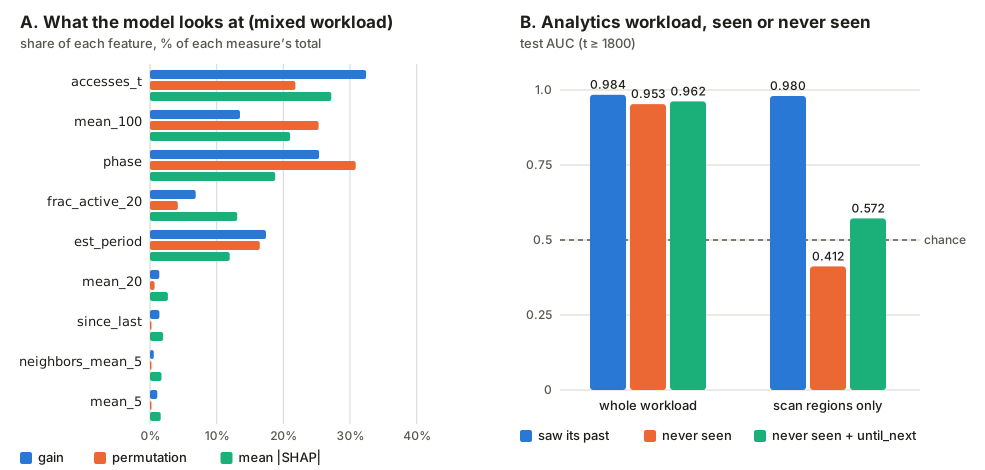
The three measures disagree on the ranking. est_period is the most used feature (30.6% of splits) but only fifth by SHAP: it’s a continuous variable with many thresholds, which the split count rewards. accesses_t is used in 2.6% of splits but brings 32.4% of the gain: a few splits, near the root, that do most of the work.
They agree on the essentials. Five features (accesses_t, mean_100, phase, frac_active_20, est_period) carry almost everything; the other four are worth less than 3% each, whatever the measure.
since_last is not useless, it’s redundant. It’s the LRU information, and shuffling it costs 0.001 AUC. Exercise 1 shows that once accesses_t is removed, its permutation importance climbs to 0.091: the information is there, and the model just reads it elsewhere.

Partial dependence of phase (mean prediction over 20,000 test rows):

`phase`	0	0.25	0.5	0.75	0.9	1.0	1.5	2	5
PD	0.238	0.244	0.312	0.411	0.412	0.268	0.278	0.284	0.319

The model has learned a bump between 0.5 and 0.9, the same one the depth-3 tree found in part 17: “we’re getting close to the next activation”. Past 1, the cycle has been missed and the region looks cold again. Careful with the left end: phase = 0 means “accessed right now”, so forcing it on a region that has been silent for 50 aggregations creates a row that can’t exist. The 0.238 averages many such rows: it’s exactly the caveat of section 3.

Two panels. A: share of each feature in three importance measures for the LightGBM on the mixed workload; accesses_t, mean_100, phase and est_period dominate, since_last and neighbors_mean_5 are near zero. B: test AUC on the analytics workload; whole workload 0.984 (saw its past), 0.953 (never seen), 0.962 (never seen + until_next); scan regions only 0.980, 0.412 (below chance), 0.572.

Error analysis: why the scan is missed

We go back to the analytics workload of part 18 and compare two models on the same test rows: the one that never saw this workload (leave-one-workload-out) and the one that saw its past (in-workload).

# 2. Error analysis: where does the model that never saw "analytics" go wrong?
ana = after[after.workload == "analytics"].copy()
ana["kind"] = np.where(ana.t < T_CHANGE, kinds_ana[ana.region, 0], kinds_ana[ana.region, 1])
lowo = fit(before[before.workload != "analytics"])     # never saw this workload
in_wl = fit(before[before.workload == "analytics"])    # saw its past


def row_log_loss(y, p):
    p = np.clip(p, 1e-7, 1 - 1e-7)
    return -(y * np.log(p) + (1 - y) * np.log(1 - p))


for name, m in [("lowo", lowo), ("in", in_wl)]:
    ana["p_" + name] = m.predict_proba(ana[FEATURES])[:, 1]
    ana["loss_" + name] = row_log_loss(ana.y, ana["p_" + name])
ana["excess"] = ana.loss_lowo - ana.loss_in            # what not having seen the workload costs


def auc_by_kind(col):
    return ana.groupby("kind").apply(lambda d: roc_auc_score(d.y, d[col]) if d.y.nunique() > 1 else np.nan)


g = ana.groupby("kind")
print(pd.DataFrame({"rows": g.size(), "positives": g.y.mean(),
                    "AUC lowo": auc_by_kind("p_lowo"), "AUC in": auc_by_kind("p_in"),
                    "excess loss": g.excess.sum()}).round(3))
regions = ana.groupby("region").agg(kind=("kind", "last"), mean_loss=("loss_lowo", "mean"),
                                    excess=("excess", "sum"))
print("20 worst regions, by mean loss:", regions.nlargest(20, "mean_loss").kind.value_counts().to_dict())
print("20 worst regions, by excess:   ", regions.nlargest(20, "excess").kind.value_counts().to_dict())

# What does SHAP say about scan regions just before they're read?
scan = ana[(ana.kind == "scan") & (ana.y == 1)]
c = lowo.booster_.predict(scan[FEATURES], pred_contrib=True)
print(f"scan, y = 1: mean p {scan.p_lowo.mean():.3f} (in-workload model: {scan.p_in.mean():.3f}), {len(scan)} rows")
print("medians:", scan[["since_last", "est_period", "phase", "mean_100", "frac_active_20"]].median().to_dict())
print("mean SHAP:", dict(zip(FEATURES, c[:, :-1].mean(0).round(3))), "| phi_0", round(c[0, -1], 3))

Behavior	Rows	Positives	AUC never seen	AUC saw its past	Excess loss
bursty	8,320	28.8%	0.676	0.684	+233
cold	10,720	9.2%	0.513	0.500	−269
hot	36,920	99.9%	0.549	0.555	+129
periodic	13,080	36.2%	0.985	0.931	−2,466
scan	45,200	4.7%	0.412	0.980	+8,560

The scan explains everything, and more. The total excess is +6,187; the scan alone weighs +8,560. Elsewhere, the model that never saw the workload does better on periodic regions (0.985 vs 0.931): it was trained on jvm, 70% periodic, so it saw many more cycles.
On scan regions, AUC 0.412 is below chance. The model ranks “about to be read” regions below “silent” ones. It’s not that it doesn’t know; it’s confidently wrong.
Sorting by raw loss points elsewhere. The 20 regions with the highest mean loss are 8 bursty, 6 cold and 6 scan: bursts are hard for every model. Sorting by excess, all 20 are scan regions. That’s the reason for step 2 of the procedure.
The AUCs of hot and cold mean little. 99.9% positives on one side, Poisson accesses at 0.01 on the other: there’s almost nothing to rank there.

What SHAP says about scan regions just before they’re read (2,126 rows with $y = 1$ ): the model gives them on average 0.166, versus 0.853 for the in-workload model. Their medians: since_last 232, est_period 240, phase 0.975, mean_100 0 and frac_active_20 0. Mean contributions:

Feature	Mean $\phi_j$
`mean_100`	−0.545
`frac_active_20`	−0.399
`est_period`	−0.190
`since_last`	−0.095
`phase`	+0.196

The diagnosis reads directly: phase says “it’s coming” (0.975, right in the bump), but the model has only seen cycles of 15 to 60 aggregations. For it, a region silent for 100 aggregations (mean_100 = 0, frac_active_20 = 0) and with a period of 240 is a cold region, and those two signals win. The useful information was there; it was just expressed relative to the period, whereas the label is defined in absolute time ( $H = 10$ aggregations).

A feature in the label’s units

Hence the idea: the number of aggregations remaining before the next expected start, until_next = est_period − since_last. For a periodic region with a period of 30 or a scan with a period of 240, “until_next between 1 and 10” means the same thing: activation falls within the label window. A tree trained on periodic regions learns that threshold, and it transfers to the scan without having seen it.

We decide on the validation (training $t < 1390$ , validation $1400 \le t < 1790$ , part 15’s split), then confirm once on the test.

# 3. A feature in the label's units: aggregations until the next expected start
everything["until_next"] = everything.est_period - everything.since_last
F2 = FEATURES + ["until_next"]

# a) Decide without touching the test: train t < 1390, validation 1400 <= t < 1790
tr = everything[everything.t < 1390]
va = everything[(everything.t >= 1400) & (everything.t < 1790) & (everything.workload == "analytics")]
for feats in (FEATURES, F2):
    m = fit(tr[tr.workload != "analytics"], feats)
    print(f"{len(feats)} features | validation, analytics never seen: "
          f"{roc_auc_score(va.y, m.predict_proba(va[feats])[:, 1]):.3f}")

# b) Confirm once on the test, with part 18's three protocols
before, after = everything[everything.t < t_test - H], everything[everything.t >= t_test]
for name in workloads:
    te = after[after.workload == name]
    row = []
    for feats in (FEATURES, F2):
        for d in (before[before.workload == name], before[before.workload != name], before):
            row.append(roc_auc_score(te.y, fit(d, feats).predict_proba(te[feats])[:, 1]))
    print(f"{name:>9} | 9 features {np.round(row[:3], 3)} | + until_next {np.round(row[3:], 3)}")

# And on the scan regions alone, for the model that never saw them
te = after[after.workload == "analytics"].assign(kind=ana.kind.values)
m = fit(before[before.workload != "analytics"], F2)
s = te.kind == "scan"
print(f"scan only, never seen: AUC {roc_auc_score(te.y[s], m.predict_proba(te[F2][s])[:, 1]):.3f}")

On the validation, the model that never saw the analytics workload goes from 0.964 to 0.971 with until_next: we keep the feature. Confirmation on the test, with part 18’s three protocols:

Workload	In-workload	Never seen	Three workloads	In-workload + `until_next`	Never seen + `until_next`	Three + `until_next`
mixed	0.873	0.865	0.874	0.875	0.868	0.879
jvm	0.980	0.980	0.985	0.985	0.983	0.986
analytics	0.984	0.953	0.988	0.985	0.962	0.988

The feature helps everywhere, and especially where it was meant to. Never-seen analytics goes from 0.953 to 0.962: it recovers almost a third of the 3.1 points lost. No cell gets worse.
But it doesn’t solve the scan. On scan regions alone, AUC rises from 0.412 to 0.572, far from the 0.980 of a model that saw scans. A good feature makes the information readable; it doesn’t replace having seen the behavior.
The gain is confirmed by the folds. In part 18’s time-based cross-validation on the mixed workload, until_next improves all four folds (exercise 3). A gain that only showed up on the test would have been suspect.

Running project: what this changes for the thesis

Q1 and H1 now have a method. “Are periodicity and neighborhood the most predictive features?” is answered with the three measures side by side, on held-out data, not with LightGBM’s default importance (split count). On our simulation: periodicity, yes (phase + est_period weigh 47% of permutation importance and 31% of mean |SHAP|), neighborhood, no (neighbors_mean_5 weighs at most 2.3% of splits and under 2% on the other three measures). Caution: this verdict is the simulation’s, where neighbors share the same kind but not the same phase. Only real DAMON traces can settle H1.
Report importances with their limits. Always note the redundant groups (accesses_t / since_last / phase): a “useless” feature in permutation can be the only one left if you remove its twin. Exercise 1 gives the numbers.
Error analysis is a chapter, not an appendix. The excess-loss table per behavior, with the SHAP explanation of the guilty slice, is exactly the kind of result a committee expects: it says why the model fails, not just how much.
Express the features in the label’s units. The horizon $H$ will be a parameter of the daemon (how far ahead to protect a page from zswap). Features measured in the same unit (until_next) generalize better than relative features (phase) when the periods change from one workload to another.
For the LSTM (part 23), SHAP still applies (shap.DeepExplainer, or integrated gradients), but TreeSHAP’s exactness is lost. That’s an argument in favor of LightGBM if both models end up with similar scores.

Hands-on exercise

Correlated features. Retrain the mixed-workload model without accesses_t, then recompute the permutation importance. What happens to the AUC? And to the importance of since_last? What does this tell you about the sentence “this feature is useless”?
Check against the shap library. Install shap and compute shap.TreeExplainer(model).shap_values(sample[FEATURES]). Compare with phi (largest absolute difference) and with the computation time of pred_contrib.
Confirm in cross-validation. Reuse part 18’s time_folds and cv_score (with P and the mixed workload’s development period) to compare FEATURES and F2 fold by fold. Is the gain positive on all four folds? Is it larger than the spread across folds?
A neighborhood feature for the scan. In a scan, the regions before reg are read just before it. Build upstream_mean_5, the mean of the rolling-5 activity of regions reg - 4 to reg - 1, add it to F2, and measure never-seen analytics. Explain the result with what this article showed.
Running project. For each of your real workloads, produce the excess-loss table per slice. With no “true kind” available on DAMON traces, which slices would you use? (Hint: address ranges, est_period buckets, before/after a known phase change of the program.)

Hints. Question 1: AUC 0.873 → 0.872; the permutation importance of since_last goes from 0.001 to 0.091. Question 2: largest difference 0.0 (identical values); on our two-core machine, about 7 s for 20,000 rows in both cases (6.96 s with pred_contrib, 7.38 s with shap). Question 3: 0.9052 · 0.8998 · 0.9073 · 0.9190 (mean 0.9078) → 0.9063 · 0.9041 · 0.9076 · 0.9194 (mean 0.9093); a gain of 0.0011 · 0.0043 · 0.0003 · 0.0004, positive on all four folds but smaller than the standard deviation across folds. Question 4: 0.962 → 0.962, no gain: the model never saw a case where upstream activity announces a read, so it hasn’t learned to use it. Only training data containing scans would make this feature useful.

Further resources

Lundberg and Lee, A Unified Approach to Interpreting Model Predictions (NeurIPS 2017): SHAP and its properties.
Lundberg et al., From local explanations to global understanding with explainable AI for trees (Nature Machine Intelligence, 2020): exact TreeSHAP.
Christoph Molnar, Interpretable Machine Learning, chapters on permutation importance, partial dependence and Shapley values.
scikit-learn docs: Permutation feature importance (section on correlated features) and Partial Dependence and Individual Conditional Expectation plots.
Refresher: M7 · Random variables, distributions, expectation and variance, for $\phi_0 = \mathbb{E}[f(X)]$ .

What you should be able to do before moving on

Explain the difference between gain, split count and permutation importance, and the bias of each
Explain why a redundant feature looks useless in permutation importance
State the efficiency property of Shapley values and check it on a LightGBM model
Compute SHAP values with pred_contrib=True and read them locally and globally
Compute a partial dependence curve and spot the impossible rows it creates
Run an error analysis by slices, with an excess loss against a reference model
Propose a feature from a diagnosis and validate it without touching the test

Next part: Unsupervised learning: exploring without labels (part 20). Here we cheated: we knew each region’s true kind. On real DAMON traces we won’t; we’ll see how clustering can find those behavior families from the access traces alone, and even spot a new behavior before the model gets it wrong.