Linear models and regularization

Mastering AI · Technical phase · Week 1 · Part 16

Goal of this step

In parts 14 and 15, logistic regression was just one row in a table, beaten by gradient boosting. Yet it’s the thesis’s first baseline, and not out of politeness: it fits in a dozen multiplications, its weights can be read, and it runs comfortably inside a system daemon. Before replacing it with something bigger, you need to know exactly what it does.

By the end of this article you’ll be able to:

• go from a linear score to a probability with the sigmoid, and read a coefficient as an effect on the odds;
• explain why we train with log-loss and not with MSE;
• tune $L_1$ / $L_2$ regularization with scikit-learn’s C, and understand why C has to be so small;
• help a linear model with transformed features, and see where that stops being enough;
• compute the real inference cost of a logistic regression in production.

---

Key concepts

1. From linear to logistic regression

Intuition. The linear regression from the low-level article outputs any number. For a probability, we need to squash it between 0 and 1: that’s the job of the sigmoid.

$$z = w^\top x + b \qquad p = \sigma(z) = \frac{1}{1 + e^{-z}}$$

Inverting it gives the form that makes coefficients readable:

$$\log \frac{p}{1 - p} = w^\top x + b$$

The left-hand side is the log of the odds (the logit). So the model is linear, but in log-odds. Practical consequence: if feature $x_j$ increases by 1, the odds $p / (1 - p)$ are multiplied by $e^{w_j}$ , all other features held fixed.

2. Why log-loss and not MSE

Intuition. When the model is confidently wrong, we want it to feel it strongly. With MSE passed through a sigmoid, it’s the opposite: the more confidently wrong it is, the smaller the gradient.

Log-loss (or binary cross-entropy) is the negative likelihood from Required Maths M8:

$$\mathcal{L}(w, b) = -\frac{1}{n} \sum_{i=1}^{n} \Big[ y_i \log p_i + (1 - y_i) \log (1 - p_i) \Big]$$

Its derivative with respect to the score is remarkably simple, while MSE’s drags a factor $p(1 - p)$ that vanishes at the extremes:

$$\frac{\partial \ell_{\log}}{\partial z} = p - y \qquad \frac{\partial (p - y)^2}{\partial z} = 2 (p - y) \, p (1 - p)$$

As a bonus, log-loss is convex in $(w, b)$ : its Hessian is $X^\top D X$ , with $D$ diagonal with entries $p_i (1 - p_i) \ge 0$ , so it’s positive semi-definite (Required Maths M6). No local-minimum trap: any solver finds the optimum.

3. $L_2$ and $L_1$ regularization, and the C trap

Intuition. We add a penalty on the size of the weights. $L_2$ shrinks them all a bit; $L_1$ sets some of them exactly to zero, which performs feature selection. The geometry (round ball versus diamond) is in Required Maths M11.

Practical trap: scikit-learn doesn’t minimize “mean loss $+ \lambda \times$ penalty”, but a sum of losses multiplied by C:

$$\min_{w, b} \; \frac{1}{2} \lVert w \rVert_2^2 + C \sum_{i=1}^{n} \ell_i \qquad \text{or} \qquad \min_{w, b} \; \lVert w \rVert_1 + C \sum_{i=1}^{n} \ell_i$$

Dividing by $C n$ gives back the textbook form with $\lambda = 1 / (C n)$ . With our $n = 123{,}840$ training examples, C = 1 corresponds to $\lambda \approx 8 \times 10^{-6}$ : almost no regularization. To see an effect, you have to go down to C $\approx 10^{-4}$ , i.e. $\lambda \approx 0.08$ .

4. Scaling to read the coefficients

Intuition. A weight depends on its feature’s unit. since_last goes from 0 to 500, frac_active_20 from 0 to 1: their raw weights aren’t comparable. After a StandardScaler, each weight reads as “effect on the log-odds of an increase of one standard deviation”.

Two warnings:

• scaling is also essential for regularization, otherwise the penalty hits small-scale features harder;
• a coefficient is an effect all else being equal. When features are highly correlated (our three rolling means), that scenario barely exists in the data, and the signs can be surprising. We’ll see it below.

5. What a linear model cannot see

Intuition. The log-odds are a monotonic function of each feature. But some effects aren’t. For a periodic region, the dangerous moment is when phase is close to 1 (the cycle is about to restart): not too early, not too late. A single weight on phase cannot express “close to 1”.

Two solutions: build features that make the effect monotonic (a logarithm, a bump around 1), or switch to a non-linear model (trees, part 17). The first keeps the model lightweight.

6. Inference cost

Intuition. In production, we don’t even need the sigmoid. Since $\sigma$ is increasing, $p \ge s \iff z \ge \operatorname{logit}(s)$ . So we compare $w^\top x + b$ directly with a precomputed threshold, and we can fold the scaling into the weights:

$$w_j^{\text{raw}} = \frac{w_j}{\sigma_j} \qquad b^{\text{raw}} = b - \sum_j \frac{w_j \, \mu_j}{\sigma_j}$$

where $\mu_j$ and $\sigma_j$ are the mean and standard deviation learned by the scaler. For $d$ features: $d$ multiplications, $d$ additions and one comparison per region.

---

Code example

We reuse the part 14 script as is (simulation, features, labels), then append the five blocks below in the same file. The split is the one from part 15: train $t < 1390$ , validation $1400 \le t < 1790$ , test $t \ge 1800$ (with the regime change at $t = 2100$ ). The whole thing runs in about ten seconds.

The baseline and its coefficients

# Continues the part 14 script: df, FEATURES, H, np, pd, make_pipeline, StandardScaler,
# LogisticRegression, HistGradientBoostingClassifier and roc_auc_score are already defined.
import time
from sklearn.metrics import average_precision_score, log_loss

# Same three periods as in part 15
t_val, t_test = 1400, 1800
train = df[df.t < t_val - H]
val = df[(df.t >= t_val) & (df.t < t_test - H)]
test = df[df.t >= t_test]

# 1. The baseline: standardization + logistic regression (L2, C = 1)
lr = make_pipeline(StandardScaler(), LogisticRegression(C=1.0, max_iter=1000))
lr.fit(train[FEATURES], train.y)
p_val = lr.predict_proba(val[FEATURES])[:, 1]
print(f"logistic, validation: AUC {roc_auc_score(val.y, p_val):.3f} | "
      f"AP {average_precision_score(val.y, p_val):.3f} | log-loss {log_loss(val.y, p_val):.3f}")

w = lr[-1].coef_[0]
coefs = pd.DataFrame({"w (per std)": w, "odds x": np.exp(w)}, index=FEATURES)
print(coefs.sort_values("w (per std)", key=abs, ascending=False).round(2))
print(f"intercept b = {lr[-1].intercept_[0]:.2f} | corr(mean_20, y) on train = {train.mean_20.corr(train.y):.2f}")

On validation: AUC 0.808, average precision 0.725, log-loss 0.447.

Feature	$w$ (per std)	Odds multiplied by $e^{w}$
frac_active_20	1.77	5.90
mean_20	−1.36	0.26
accesses_t	0.80	2.23
mean_100	0.80	2.23
mean_5	−0.32	0.73
est_period	−0.31	0.73
since_last	−0.10	0.91
phase	−0.07	0.93
neighbors_mean_5	0.06	1.06

The intercept is $b = -0.81$ .

• The strongest feature is regularity: one more standard deviation of frac_active_20 multiplies the odds of being hot by 5.9.
• mean_20 has a negative weight, even though on its own it’s positively related to heat (correlation 0.38 on train). That’s not a bug: the weight measures the effect of mean_20 with mean_5, mean_100 and frac_active_20 held fixed, a rare situation since these means move together. The model uses it as a correction term between time scales, not as a heat indicator. That’s the warning from concept 4: you don’t read a coefficient in isolation when features are correlated.

Log-loss versus MSE, in numbers

# 2. Why log-loss rather than MSE: the gradient for a confidently wrong prediction
z = np.array([-6.0, -2.0, 0.0, 2.0])     # score of a region that is actually hot (y = 1)
p = 1 / (1 + np.exp(-z))
grad_logloss = p - 1                       # d/dz of -log(p)
grad_mse = 2 * (p - 1) * p * (1 - p)       # d/dz of (p - 1)^2
for zi, pi, gl, gm in zip(z, p, grad_logloss, grad_mse):
    print(f"z = {zi:+.0f} | p = {pi:.3f} | gradient log-loss {gl:+.3f} | gradient MSE {gm:+.4f}")

$z$ (actually hot region)	$p$	Log-loss gradient	MSE gradient
−6	0.002	−0.998	−0.0049
−2	0.119	−0.881	−0.1850
0	0.500	−0.500	−0.2500
+2	0.881	−0.119	−0.0250

For the worst error ( $z = -6$ , the model is 99.8% sure the region is cold), log-loss pushes with a force of almost 1. MSE pushes 200 times less: it leaves the model in its error. That’s exactly the case we want to fix first, since a false cold is expensive.

$L_1$ and $L_2$ regularization paths

# 3. L1 versus L2: which features survive when the penalty grows?
print(f"{len(train)} training examples")
for C in np.logspace(-5, -2, 7):
    for name, l1_ratio in (("L1", 1.0), ("L2", 0.0)):
        m = make_pipeline(StandardScaler(),
                          LogisticRegression(C=C, l1_ratio=l1_ratio, solver="saga", max_iter=5000))
        m.fit(train[FEATURES], train.y)
        w_c = m[-1].coef_[0]
        auc_c = roc_auc_score(val.y, m.predict_proba(val[FEATURES])[:, 1])
        kept = [f for f, wi in zip(FEATURES, w_c) if wi != 0]
        print(f"C = {C:.1e} | {name} | non-zero: {len(kept)} | |w| sum {np.abs(w_c).sum():.2f} | "
              f"AUC val {auc_c:.3f}" + (f" | {kept}" if name == "L1" and len(kept) < 9 else ""))

C	$L_1$ : non-zero features	$L_1$ : val AUC	$L_2$ : val AUC
$10^{-5}$	0	0.500	0.769
$3.2 \times 10^{-5}$	0	0.500	0.774
$10^{-4}$	3	0.780	0.783
$3.2 \times 10^{-4}$	6	0.786	0.796
$10^{-3}$	8	0.799	0.806
$3.2 \times 10^{-3}$	9	0.808	0.809
$10^{-2}$	9	0.809	0.809

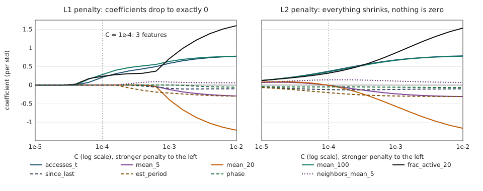
• At C = 1e-4, $L_1$ keeps only three features: accesses_t (the present), mean_100 (the long term) and frac_active_20 (regularity). With those alone, AUC is already 0.780, versus 0.809 with all nine.
• Next come since_last, est_period and neighbors_mean_5 (6 features), then mean_5 and mean_20, and phase last. mean_20 only enters late, and that’s where it turns negative: it only serves to correct the other means.
• $L_2$ never sets anything to zero: even at C = 1e-5, all nine weights are non-zero, just small.
• Beyond C = 3e-3, nothing moves any more: with 123,840 examples and 9 features, there’s no overfitting to fight. Here, regularization mainly serves to select, not to generalize.

Helping the linear model, and comparing it with boosting

# 4. Helping a linear model: transformed features
def add_features(d):
    d = d.copy()
    d["log_since"] = np.log1p(d.since_last)               # recency acts on a log scale
    d["log_period"] = np.log1p(d.est_period)
    d["near_cycle"] = np.exp(-((d.phase - 1) / 0.2) ** 2)  # ~1 when a cycle is about to restart
    return d


FEATURES_PLUS = FEATURES + ["log_since", "log_period", "near_cycle"]
tr, va, te = add_features(train), add_features(val), add_features(test)
C_FALSE_COLD, C_FALSE_HOT = 10, 1


def average_cost(y, p, threshold):
    pred = p >= threshold
    return (C_FALSE_COLD * np.sum((y == 1) & ~pred) + C_FALSE_HOT * np.sum((y == 0) & pred)) / len(y)


thresholds = np.linspace(0.01, 0.99, 99)
candidates = {
    "logistic, 9 features": (make_pipeline(StandardScaler(), LogisticRegression(max_iter=2000)), FEATURES),
    "logistic, 12 features": (make_pipeline(StandardScaler(), LogisticRegression(max_iter=2000)), FEATURES_PLUS),
    "boosting, 9 features": (HistGradientBoostingClassifier(max_iter=200, random_state=0), FEATURES),
}
print(f"never compress: test cost {average_cost(te.y.to_numpy(), np.ones(len(te)), 0.5):.3f}")
fitted, chosen = {}, {}
for name, (m, F) in candidates.items():
    m.fit(tr[F], tr.y)
    fitted[name] = m
    pv, pt = m.predict_proba(va[F])[:, 1], m.predict_proba(te[F])[:, 1]
    s = thresholds[int(np.argmin([average_cost(va.y.to_numpy(), pv, s) for s in thresholds]))]
    chosen[name] = s
    print(f"{name:>22} | AUC val {roc_auc_score(va.y, pv):.3f} | AUC test {roc_auc_score(te.y, pt):.3f} | "
          f"threshold {s:.2f} | cost val {average_cost(va.y.to_numpy(), pv, s):.3f} | "
          f"cost test {average_cost(te.y.to_numpy(), pt, s):.3f} | compressed (test) {(pt < s).mean():.3f}")

Reference: never compressing anything costs 0.689 per region on test (and 0.699 on validation), since every cold region becomes a false hot.

Model	Val AUC	Test AUC	Threshold (val)	Val cost	Test cost	Compressed (test)
Logistic, 9 features	0.808	0.793	0.14	0.665	0.723	17.6%
Logistic, 12 features	0.832	0.806	0.05	0.676	0.694	1.5%
Boosting, 9 features	0.911	0.858	0.11	0.547	0.707	32.9%
Never compress				0.699	0.689	0%

Three lessons, one of which goes beyond this article:

• the three transformed features add 2.4 AUC points on validation (0.808 → 0.832) and 1.3 on test. near_cycle is the one that helps most, because it gives the linear model the “phase close to 1” bump it can’t build on its own;
• a better AUC doesn’t guarantee a better cost. With 12 features, the chosen threshold drops to 0.05: the model ranks better, but it doesn’t isolate a group that is “surely cold” enough to dare compressing. It compresses only 1.5% of regions, i.e. almost nothing. With a false cold at 10, what matters is the purity of the low-score zone, not the overall ranking;
• on validation, boosting clearly beats the reference (0.547 versus 0.699). On test, no model does better than “never compress” (0.689): the regime change at $t = 2100$ wakes up regions every model believed were cold. Part 15 measured a 31% cost reduction relative to the 0.5 threshold; the real reference is this one, and it’s the one the thesis will have to beat. Parts 18 (per-workload validation) and 28 (monitoring) deal with this problem.

Inference cost

# 5. Inference cost: fold the scaler into the weights, then a single dot product
best = fitted["logistic, 12 features"]
scaler, clf = best[0], best[-1]
w_raw = clf.coef_[0] / scaler.scale_                       # weights in the features' own units
b_raw = clf.intercept_[0] - np.sum(clf.coef_[0] * scaler.mean_ / scaler.scale_)
s = chosen["logistic, 12 features"]
z_star = np.log(s / (1 - s))                               # p >= s  <=>  z >= logit(s)
now = te[te.t == t_test]                                   # the 96 regions at one aggregation
X96 = now[FEATURES_PLUS].to_numpy()
same = np.allclose(X96 @ w_raw + b_raw, best.decision_function(now[FEATURES_PLUS]))
t0 = time.perf_counter()
for _ in range(10_000):
    keep = X96 @ w_raw + b_raw >= z_star
dt = (time.perf_counter() - t0) / 10_000
print(f"same scores as the pipeline: {same} | logit threshold z* = {z_star:.3f}")
print(f"{len(w_raw)} multiplications + {len(w_raw)} additions per region | "
      f"96 regions: {dt * 1e6:.1f} µs per aggregation")

• The scores computed by hand with the folded weights are identical to the scikit-learn pipeline’s.
• The 0.05 threshold becomes $z^\star = \operatorname{logit}(0.05) = -2.944$ : no exponential to compute in production.
• 12 multiplications and 12 additions per region. For the 96 regions of one aggregation, the decision takes about 2 µs in NumPy on my machine (2.1 to 2.6 µs depending on the run), compared with an aggregation period of 100 ms.

---

Running project: what this changes for the thesis

• The baseline is set. Standardized logistic regression, C chosen on validation, threshold chosen on validation with the cost $c_{FN} / c_{FP}$ stated in advance. It’s the floor: an LSTM that doesn’t clearly beat it isn’t worth its complexity.
• Inference cost is an argument. For $10^5$ DAMON regions, one decision costs about $1.2 \times 10^6$ multiply-adds per aggregation. In NumPy, on my machine, that takes about 0.4 ms (measured by repeating the 96 regions up to $10^5$ rows): compatible with a daemon running continuously; we’ll measure the same thing for LightGBM and the LSTM.
• $L_1$ as an analysis tool. The $L_1$ path gives an importance order for the features (regularity, long-term intensity, present), to compare with your hypothesis H1 on periodicity.
• The real reference is “never compress”. Every model must be compared with it, in cost, on test. We add this line to the part 15 protocol.

---

Hands-on exercise

1. $L_1$ versus noise. Add 5 Gaussian noise columns (rng.normal(size=len(d))) to train and validation, then redo the $L_1$ path. Up to which C do their weights stay exactly zero? What does that tell you about the truly useful features?
2. Collinearity. Remove mean_20 and retrain the baseline. What happens to AUC and to the weight of frac_active_20? Explain with concept 4.
3. Calibration. Compute the test Brier score for the 12-feature logistic regression and for boosting (part 15). Is the linear model better calibrated? Why does it matter for the theoretical threshold $s^\star = 1/11$ ?
4. Is the gap real? The test cost of the 12-feature logistic regression (0.694) is lower than boosting’s (0.707). Compute a 95% confidence interval on the difference with a bootstrap over regions (draw 96 regions with replacement, not rows, because rows of the same region are correlated), using the tools from Required Maths M9. Conclude.
5. Running project. Write the decision function for one region in C (or Rust): an array of 12 weights, a bias, a threshold $z^\star$ . How many bytes does the whole model take?

Hints. Question 1: with seed 1 for the noise, all five weights stay zero up to C = 1e-3; only one becomes non-zero (and tiny) at C = 1e-2. Question 2: validation AUC goes from 0.808 to 0.801 and the weight of frac_active_20 from 1.77 to 0.52. Question 3: 0.1467 versus 0.1119. Question 4: with 2,000 draws, the difference is −0.013 and the interval is about [−0.062, +0.039].

---

Further resources

• Refresher: Linear regression, low-level.
• James, Witten, Hastie, Tibshirani, An Introduction to Statistical Learning (ISLR), chapter 4 (classification, logistic regression) and chapter 6 (ridge and lasso).
• scikit-learn docs: Logistic regression (linear models section), and the example Regularization path of L1-Logistic Regression.
• Hastie, Tibshirani, Wainwright, Statistical Learning with Sparsity (2015), chapters 2 and 3: why the lasso sets weights exactly to zero.

---

What you should be able to do before moving on

• Write the logistic model and read a coefficient as a multiplicative factor on the odds
• Explain, with the gradient, why log-loss rather than MSE for classification
• Translate scikit-learn’s C into $\lambda$ , and choose between $L_1$ and $L_2$
• Read scaled coefficients without falling into the correlated-features trap
• Add a transformed feature for a non-monotonic effect
• Fold the scaler into the weights and compute the inference cost of a decision
• Compare a model with the “never compress” reference, not only with another model

Next part: Trees, forests and gradient boosting (part 17). We open up the model that has been winning since part 14: how a tree builds on its own the thresholds and bumps we had to add by hand here.