October 27, 2026 · 21 min read

A neural network by hand with PyTorch

Tensors, autograd checked by hand and a complete training loop: a PyTorch MLP on memory traces, compared with logistic regression and boosting, and three silent bugs measured.

Mastering AI · Technical phase · Week 3 · Part 21

Goal of this step

In the M12 wrap-up, you wrote an MLP entirely in NumPy: forward pass, backpropagation by hand, AdamW. It works, but every new layer means rewriting the backward pass, and the slightest index mistake gives a wrong gradient that still “learns” a little. Since part 16, we’ve been working with ready-made models (scikit-learn, LightGBM). For sequence models (part 23), we need a tool that computes gradients for you, without turning into a black box.

PyTorch is that tool. The idea of this article: delegate nothing to it that you couldn’t redo yourself. We check every gradient it computes against a gradient written by hand.

By the end of this article you’ll be able to:

handle tensors (shape, dtype, device) and relate them to what you already do in NumPy;
explain what autograd builds during the forward pass and what loss.backward() does;
check an autograd gradient against the M12 formula and with finite differences;
write a complete training loop (nn.Module, DataLoader, AdamW, validation, best epoch);
recognize, with numbers, three classic slips: zero_grad(), model.eval() and input scaling.

Key concepts

1. A tensor is a NumPy array that knows where it lives and where it comes from

Intuition. A torch.Tensor looks a lot like an np.ndarray: same shapes, same broadcasting, same @ for matrix products. It adds three things:

Attribute	What it says	Usual value here
`dtype`	the type of the numbers	`float32` (NumPy works in `float64` by default)
`device`	where the data lives	`cpu`; `cuda` on a graphics card
`requires_grad`	should operations be tracked for differentiation?	`True` for parameters

float32 halves memory and speeds up computation, at the price of about 7 significant digits instead of 16. That’s plenty for training, but not for checking a gradient with finite differences: we then switch back to float64.

A GPU would bring little to a 1,409-parameter network: with such small matrices, the cost is mostly launching operations, not computing. Everything below runs on CPU. To move to a GPU, you just move the model and the data with .to("cuda"), and nothing else changes.

2. A dense layer is an affine transformation

Intuition. A dense layer does exactly what a matrix does in Required Maths M2: it transforms space, then adds a translation. The non-linearity comes after.

h = \operatorname{ReLU}(W x + b), \qquad W \in \mathbb{R}^{n_{\text{out}} \times n_{\text{in}}}

nn.Linear(9, 32) holds a $32 \times 9$ matrix $W$ and a bias $b$ of size 32, i.e. 320 parameters. Our network chains three layers: $9 \to 32 \to 32 \to 1$ , i.e. $320 + 1{,}056 + 33 = 1{,}409$ parameters. The output is a logit $z$ , a real-valued score; the probability is $\sigma(z)$ .

3. The computation graph and autograd

Intuition. During the forward pass, PyTorch takes notes: every operation on a tensor that requires a gradient is recorded along with its inputs. At the end, loss.backward() reads those notes backwards and applies the chain rule from Required Maths M5 at each step.

For a logistic regression, the graph has three nodes: product plus bias, sigmoid, loss. Going backwards, we get back the formula written by hand in M12:

\frac{\partial \ell}{\partial w} = \frac{1}{n} X^\top (p - y)

Three rules to remember:

the graph is rebuilt at every forward pass. An if or a for loop inside forward is therefore allowed: the graph follows the path actually taken;
gradients add up in .grad instead of replacing it. That’s on purpose (a variable used twice receives the sum of its two contributions), but it means .grad must be cleared before each step;
torch.no_grad() stops the recording: for evaluation, it’s faster and doesn’t spend memory on a useless graph.

This way of computing is called reverse-mode automatic differentiation. A single backward pass gives the gradient with respect to all parameters, at a cost of the same order as a forward pass. That’s what makes it possible to train networks with millions of parameters.

4. The loss: logits, not probabilities

We could apply the sigmoid, then the log-loss. In practice, we feed the logits directly to nn.BCEWithLogitsLoss, which computes the same thing in a stable form:

\ell(z, y) = -\big[y \log \sigma(z) + (1 - y) \log(1 - \sigma(z))\big] = \log\!\big(1 + e^{z}\big) - y\,z

With $\sigma(z)$ rounded to exactly 1 in float32 (as soon as $z$ reaches about 17), $\log(1 - \sigma(z))$ is $-\infty$ . The right-hand form never has that problem. Its derivative is $\sigma(z) - y$ , M12’s “error arriving at the output”.

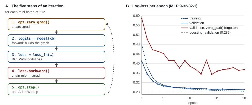
5. The training loop in five steps

Intuition. All of PyTorch’s machinery boils down to five lines, repeated for each mini-batch.

opt.zero_grad(): clear the gradients of the previous step;
logits = model(xb): forward pass, which builds the graph;
loss = loss_fn(logits, yb): a number;
loss.backward(): fills .grad of every parameter;
opt.step(): one optimizer step, here AdamW (M10 and M11).

Around it, two organizing objects: nn.Module, which holds the layers and finds their parameters by itself (model.parameters()), and DataLoader, which cuts the data into mini-batches shuffled at every epoch. And two modes: model.train() and model.eval(). They change the behavior of some layers, such as Dropout (active in training, off in evaluation) or BatchNorm. Forgetting eval() raises no error: predictions simply become random. We measure it below.

Code example

As in parts 15 to 20, we take the script from part 14 as is (simulation and dataset), then append the four blocks below. The first block doesn’t depend on the data: you can run it alone to discover PyTorch. The whole thing runs in under two minutes on a two-core CPU (numpy 2.5, pandas 3.0, scikit-learn 1.9, torch 2.14).

Tensors and autograd, checked by hand

import time
import torch
from torch import nn
from torch.utils.data import TensorDataset, DataLoader
from sklearn.metrics import log_loss

torch.manual_seed(0)
torch.set_num_threads(2)

# 1. A tensor: an array as in NumPy, plus a dtype, a device (CPU/GPU) and a history
X = torch.tensor([[1.0, 0.5], [0.2, -1.0], [-0.3, 0.8], [1.5, 1.2]])
y = torch.tensor([1.0, 0.0, 0.0, 1.0])
print(X.shape, X.dtype, X.device, "| GPU available:", torch.cuda.is_available())

# 2. A logistic regression: autograd records every operation in a graph
w = torch.zeros(2, requires_grad=True)
b = torch.zeros(1, requires_grad=True)
p = torch.sigmoid(X @ w + b)
loss = nn.functional.binary_cross_entropy(p, y)
print("loss", round(loss.item(), 4), "| graph:", loss.grad_fn.name(), "<-",
      loss.grad_fn.next_functions[0][0].name(), "<-",
      loss.grad_fn.next_functions[0][0].next_functions[0][0].name())

loss.backward()                                 # walks the graph back: chain rule (M5)
with torch.no_grad():
    print("autograd:", w.grad.numpy().round(4), "| by hand X^T(p - y)/n:", (X.T @ (p - y) / len(y)).numpy().round(4))

# 3. Gradients ACCUMULATE: a second backward adds to them
nn.functional.binary_cross_entropy(torch.sigmoid(X @ w + b), y).backward()
print("after a 2nd backward:", w.grad.numpy().round(4))
w.grad.zero_()                                  # what optimizer.zero_grad() does

# 4. Check autograd with finite differences (in float64, otherwise rounding dominates)
f = lambda w_: nn.functional.binary_cross_entropy(torch.sigmoid(X.double() @ w_), y.double())
w64 = torch.tensor([0.3, -0.7], dtype=torch.float64, requires_grad=True)
print("gradcheck:", torch.autograd.gradcheck(f, (w64,)))

Output:

torch.Size([4, 2]) torch.float32 cpu | GPU available: False
loss 0.6931 | graph: BinaryCrossEntropyBackward0 <- SigmoidBackward0 <- AddBackward0
autograd: [-0.325  -0.2375] | by hand X^T(p - y)/n: [-0.325  -0.2375]
after a 2nd backward: [-0.65  -0.475]
gradcheck: True

The graph is readable: the loss comes from a sigmoid, which comes from an addition (the bias), itself fed by the product X @ w. That’s the list of links in the chain rule.
Autograd recovers the M12 formula exactly: $X^\top(p - y)/n$ .
A second backward() doubles the gradient instead of replacing it. Remember this line: it explains the worst bug of the next section.
gradcheck compares autograd’s gradient with centered finite differences (M4), in float64. True means “they agree within tolerance”.

The data as tensors, and M12’s MLP checked against autograd

We reuse the split from part 15: training $t < 1390$ , validation $1400 \le t < 1790$ , test $t \ge 1800$ . The features are very skewed (since_last goes from 0 to 500): we apply log1p, then a standardization whose mean and standard deviation come from the training set only (part 14’s anti-leakage rule).

# Part 15's split: training t < 1390, validation 1400 <= t < 1790, test t >= 1800
tr = df[df.t < 1390]
va = df[(df.t >= 1400) & (df.t < 1790)]
te = df[df.t >= 1800]


def tensors(d, log=True, standardize=True):
    """Features -> float32 tensor. log1p squashes the tails; standardization only uses the train set."""
    A, R = d[FEATURES], tr[FEATURES]
    if log:
        A, R = np.log1p(A), np.log1p(R)
    if standardize:
        A = (A - R.mean()) / R.std()
    return (torch.tensor(A.to_numpy(), dtype=torch.float32),
            torch.tensor(d.y.to_numpy(), dtype=torch.float32))


Xtr, ytr = tensors(tr)
Xva, yva = tensors(va)
Xte, yte = tensors(te)
print(tuple(Xtr.shape), tuple(Xva.shape), tuple(Xte.shape), Xtr.dtype)

# M12's MLP (9 -> 32 -> 1), gradient written by hand, then compared with autograd
D, C = len(FEATURES), 32
g = torch.Generator().manual_seed(0)
W1 = torch.randn(D, C, generator=g) * np.sqrt(2 / D)     # He initialization (M12)
b1 = torch.zeros(C)
w2 = torch.randn(C, generator=g) * np.sqrt(2 / C)
b2 = torch.zeros(1)
Xb, yb = Xtr[:512], ytr[:512]

z1 = Xb @ W1 + b1                        # M2: affine transformation
h = torch.relu(z1)                       # non-linearity
p = torch.sigmoid(h @ w2 + b2)
d2 = (p - yb) / len(yb)                  # M5: the error arriving at the output
grad_hand = [Xb.T @ (torch.outer(d2, w2) * (z1 > 0)),   # back through w2, then ReLU's derivative
             (torch.outer(d2, w2) * (z1 > 0)).sum(0), h.T @ d2, d2.sum(0, keepdim=True)]

params = [t.clone().requires_grad_() for t in (W1, b1, w2, b2)]
W1a, b1a, w2a, b2a = params
pa = torch.sigmoid(torch.relu(Xb @ W1a + b1a) @ w2a + b2a)
nn.functional.binary_cross_entropy(pa, yb).backward()
print(f"hand / autograd gap: {max((q.grad - m).abs().max().item() for q, m in zip(params, grad_hand)):.1e}")

Output: (123840, 9) (37440, 9) (114240, 9) torch.float32, then hand / autograd gap: 6.0e-08.

The $6 \times 10^{-8}$ gap is float32 rounding, not a formula mistake: in float64, the finite-difference check of exercise 1 goes down to $6 \times 10^{-11}$ . The gradients written by hand in M12 and autograd’s are therefore the same. From here on, we can let autograd do the work, knowing exactly what it computes.

The training loop, and an honest comparison

from sklearn.metrics import roc_auc_score


class MLP(nn.Module):
    """9 -> 32 -> 32 -> 1. nn.Module registers the layers' parameters by itself."""
    def __init__(self, d_in, hidden=32, p_dropout=0.0):
        super().__init__()
        self.net = nn.Sequential(
            nn.Linear(d_in, hidden), nn.ReLU(), nn.Dropout(p_dropout),
            nn.Linear(hidden, hidden), nn.ReLU(), nn.Dropout(p_dropout),
            nn.Linear(hidden, 1))

    def forward(self, x):
        return self.net(x).squeeze(-1)           # logits: the sigmoid lives in the loss


def evaluate(model, X, y):
    model.eval()                                 # Dropout off (and BatchNorm frozen)
    with torch.no_grad():                        # no graph: faster, less memory
        p = torch.sigmoid(model(X)).numpy()
    return roc_auc_score(y.numpy(), p), log_loss(y.numpy(), p)


def train(Xtr, ytr, Xva, yva, epochs=20, seed=0, zero_grad=True, p_dropout=0.0, verbose=False):
    torch.manual_seed(seed)
    model = MLP(Xtr.shape[1], p_dropout=p_dropout)
    opt = torch.optim.AdamW(model.parameters(), lr=1e-3, weight_decay=1e-4)   # M10 + M11
    loss_fn = nn.BCEWithLogitsLoss()             # sigmoid + log-loss, numerically stable
    loader = DataLoader(TensorDataset(Xtr, ytr), batch_size=512, shuffle=True)
    best, state, hist = np.inf, None, []
    for epoch in range(1, epochs + 1):
        model.train()
        total = 0.0
        for xb, yb in loader:
            if zero_grad:
                opt.zero_grad()                  # 1. clear the gradients of the previous step
            loss = loss_fn(model(xb), yb)        # 2. forward + 3. loss
            loss.backward()                      # 4. backward: fills .grad of every parameter
            opt.step()                           # 5. one AdamW step
            total += loss.item() * len(yb)
        auc_va, ll_va = evaluate(model, Xva, yva)
        hist.append((epoch, total / len(ytr), ll_va, auc_va))
        if ll_va < best:                         # keep the best epoch on validation
            best, state = ll_va, {k: v.clone() for k, v in model.state_dict().items()}
        if verbose and epoch in (1, 2, 5, 10, 15, 20):
            print(f"epoch {epoch:>2} | train log-loss {total / len(ytr):.4f} | val {ll_va:.4f} | val AUC {auc_va:.3f}")
    model.load_state_dict(state)
    return model, hist


t0 = time.perf_counter()
model, hist = train(Xtr, ytr, Xva, yva, verbose=True)
best = min(hist, key=lambda r: r[2])
print(f"{sum(q.numel() for q in model.parameters())} parameters | {time.perf_counter() - t0:.0f} s | "
      f"best epoch {best[0]} (val log-loss {best[2]:.4f})")

# Only once on the test set, with two baselines trained on the same split
lr = make_pipeline(StandardScaler(), LogisticRegression(max_iter=1000)).fit(tr[FEATURES], tr.y)
hgb = HistGradientBoostingClassifier(max_iter=200, random_state=0).fit(tr[FEATURES], tr.y)
model.eval()
with torch.no_grad():
    p_mlp = {"va": torch.sigmoid(model(Xva)).numpy(), "te": torch.sigmoid(model(Xte)).numpy()}
probs = {"logistic regression": {k: lr.predict_proba(d[FEATURES])[:, 1] for k, d in (("va", va), ("te", te))},
         "boosting (part 15)": {k: hgb.predict_proba(d[FEATURES])[:, 1] for k, d in (("va", va), ("te", te))},
         "PyTorch MLP": p_mlp}


def average_cost(y, p, threshold, c_fn=10, c_fp=1):
    """Part 15's cost: a false cold costs 10, a false hot 1."""
    return (c_fn * np.sum((y == 1) & (p < threshold)) + c_fp * np.sum((y == 0) & (p >= threshold))) / len(y)


thresholds = np.linspace(0.01, 0.99, 99)
print(f"never compress: test cost {average_cost(te.y.to_numpy(), np.ones(len(te)), 0.5):.3f}")
for name, p in probs.items():
    s = thresholds[np.argmin([average_cost(va.y.to_numpy(), p["va"], s) for s in thresholds])]   # chosen on validation
    print(f"{name:>20} | val AUC {roc_auc_score(va.y, p['va']):.3f} | test AUC {roc_auc_score(te.y, p['te']):.3f}"
          f" | test log-loss {log_loss(te.y, p['te']):.4f} | threshold {s:.2f}"
          f" | test cost {average_cost(te.y.to_numpy(), p['te'], s):.3f} | compressed {(p['te'] < s).mean():.1%}")

Epoch	Training log-loss	Validation log-loss	Validation AUC
1	0.4793	0.4101	0.851
2	0.3879	0.3558	0.873
5	0.3099	0.3058	0.899
10	0.2931	0.2965	0.902
15	0.2867	0.2918	0.904
20	0.2836	0.2901	0.906

1,409 parameters, 17 seconds of training. The best epoch is the last one: in 20 epochs, validation hasn’t started going back up yet. The two curves stay glued together (panel B of the figure): no overfitting at this stage, which is expected with 123,840 examples for 1,409 parameters.

Then, only once, the test set, with two baselines trained on exactly the same rows. As in part 16, we don’t stop at AUC: we choose the threshold on validation with part 15’s cost (a false cold costs 10, a false hot 1), and we compare with the real reference, “never compress”, which costs 0.689 per region on test.

Model	Val AUC	Test AUC	Test log-loss	Threshold (val)	Test cost	Compressed (test)
Logistic regression (part 16)	0.808	0.793	0.4621	0.14	0.723	17.6%
Boosting (part 15)	0.911	0.858	0.3717	0.11	0.707	32.9%
PyTorch MLP	0.906	0.868	0.3502	0.08	0.653	21.0%
Never compress					0.689	0%

The MLP does much better than logistic regression (+7.5 test AUC points) with the same 9 features: its hidden layers build by themselves the non-linear transformations part 16 had to add by hand (near_cycle, log_since). That’s M12’s result, at the scale of the real dataset.
It’s slightly behind boosting on validation, but ahead on the test set (0.868 vs 0.858), with a lower log-loss (0.350 vs 0.372). The test set contains the regime change at $t = 2100$ ; a smooth function seems to depend less on the thresholds learned before the change.
Above all, it’s the only one of the three to go below “never compress”: 0.653 vs 0.689, compressing 21% of regions. The LightGBM chosen in part 17 got there too (0.666), with a non-significant gap. Here too, caution: on a single seed, the confidence interval of the gain touches zero, and the boosting we compare with isn’t tuned. Exercise 3 tests five seeds and runs the bootstrap; the serious comparison with the tuned LightGBM from part 18 will happen in the running project (part 24), with part 18’s protocol.

Three classic slips, measured

These bugs raise no error. The code runs, the loss goes down, and the model is simply worse. The only way to see them is to measure them.

# 4. Three classic slips, measured: same network, same seed, same 20 epochs
variants = {
    "reference (log1p + standardization)": (Xtr, Xva, Xte, {}),
    "standardization without log1p": (*[tensors(d, log=False)[0] for d in (tr, va, te)], {}),
    "no scaling at all": (*[tensors(d, log=False, standardize=False)[0] for d in (tr, va, te)], {}),
    "zero_grad() forgotten": (Xtr, Xva, Xte, {"zero_grad": False}),
}
for name, (A, B, Cte, options) in variants.items():
    m, _ = train(A, ytr, B, yva, **options)
    print(f"{name:>36} | val AUC {evaluate(m, B, yva)[0]:.3f} | test AUC {evaluate(m, Cte, yte)[0]:.3f}")

# Dropout: forgetting model.eval() makes predictions random
m_drop, _ = train(Xtr, ytr, Xva, yva, p_dropout=0.2)
m_drop.train()                                   # the slip: predicting in training mode
with torch.no_grad():
    p1, p2 = torch.sigmoid(m_drop(Xte)), torch.sigmoid(m_drop(Xte))
print(f"dropout 0.2 | same input, two calls: max gap {(p1 - p2).abs().max():.3f} | "
      f"test AUC in train mode {roc_auc_score(yte.numpy(), p1.numpy()):.3f} | "
      f"in eval mode {evaluate(m_drop, Xte, yte)[0]:.3f}")

# Latency: one decision for 96 regions, as the daemon would do every 100 ms
x96 = Xte[:96]
model.eval()
with torch.inference_mode():
    for _ in range(100):
        model(x96)                               # warm-up
    t0 = time.perf_counter()
    for _ in range(1000):
        model(x96)
print(f"96 regions: {(time.perf_counter() - t0) / 1000 * 1e6:.0f} µs per call")

Variant (same seed, 20 epochs)	Val AUC	Test AUC
Reference (`log1p` + standardization)	0.906	0.868
Standardization without `log1p`	0.907	0.867
No scaling at all	0.895	0.864
`zero_grad()` forgotten	0.858	0.828

Then, with a network that contains dropout (0.2): the same test batch passed twice in train() mode gives probabilities that differ by up to 0.950 for the same region, and the test AUC drops from 0.868 (eval() mode) to 0.862.

Forgetting zero_grad() is the worst: −4 test AUC points. Each step uses the sum of all gradients since the start of training, a “momentum” that never forgets and that the optimizer didn’t plan for. The red curve in the figure never goes down steadily.
Forgetting eval() makes the model random: two calls on the same input, two answers that can range from a “surely cold” region to a “surely hot” one. For the daemon, that would be a page compressed then decompressed at random.
Scaling matters less than people say, here. Without any normalization, we lose 1.1 validation points and 0.4 test points. AdamW divides each step by the recent magnitude of each parameter’s gradient, which partly compensates for differences in scale. With plain gradient descent, the effect is stronger: that’s exercise 2. As for log1p, it changes nothing here (0.907 vs 0.906), but it costs nothing and protects against extreme values.

Latency. A decision for 96 regions takes between 30 and 40 µs on our two-core CPU (34, 36 and 39 µs over three full runs of the script, 28 µs measured in isolation). That’s the same order of magnitude as the 10-tree LightGBM from part 17, and thousands of times less than DAMON’s aggregation period (100 ms).

Running project: what this changes for the thesis

The MLP becomes one more baseline. With the same features and the same split, it beats logistic regression by far, competes with boosting, and goes below “never compress” on all five seeds tested. For the Experiments chapter, the question is therefore no longer “can a network learn this problem?” but “does a sequential architecture (LSTM, part 23) bring anything beyond an MLP on the same features?”. That’s the right baseline for an LSTM: if the LSTM doesn’t beat this MLP, sequence memory brings nothing.
Check your gradients once, then trust them. If you write a custom layer or loss (for example an asymmetric loss that penalizes false colds more, like part 15’s cost), run it through torch.autograd.gradcheck in float64 before using it.
The three slips go into your code-review checklist. zero_grad() in the loop, eval() + no_grad() (or inference_mode()) at every evaluation, normalization statistics computed on the training set only and saved with the model: the daemon will have to apply exactly the same ones.
Latency is not an obstacle. A few tens of microseconds for 96 regions leave room for thousands of regions per aggregation. The real cost will be exporting the model out of Python (TorchScript or ONNX, part 26).

Hands-on exercise

Finite differences on the MLP. After torch.manual_seed(0), create a fresh MLP and convert it to float64 (.double()), compute the loss on 256 training rows and its gradient with autograd. For the first and last element of each parameter tensor, compare with $\big(L(\theta + \varepsilon) - L(\theta - \varepsilon)\big) / 2\varepsilon$ , $\varepsilon = 10^{-6}$ . What’s the largest gap? Do it again in float32: why does the gap explode?
Without Adam. Replace AdamW with torch.optim.SGD(..., lr=0.05, momentum=0.9) and train for 20 epochs on the reference inputs, then on the raw inputs (log=False, standardize=False). Do it again with lr=0.005. What do you notice about the best step size depending on scaling?
Is the gain real? Train the MLP with seed from 0 to 4 and give, for each, the test AUC and the test cost (threshold chosen on validation). Does the MLP beat boosting (0.858) and “never compress” (0.689) every time? Then, for seed 0, compute a 95% confidence interval on the cost difference MLP − “never compress” with a bootstrap over the 96 regions (2,000 draws, as in part 16). Conclude.
Longer. Go to 60 epochs. What’s the best epoch on validation? Does overfitting appear? What do you conclude for part 22?
Running project. Rewrite the training loop without looking at this article, then compare line by line. Then measure the latency of one call for the number of regions in your real DAMON workload, on the daemon’s target machine.

Hints. Question 1: largest gap $6.3 \times 10^{-11}$ in float64, but $2.5 \times 10^{-2}$ in float32: around a loss of 0.73, two neighboring float32 values are $6 \times 10^{-8}$ apart, and a $10^{-6}$ change in one weight only moves the loss by a few of those steps: the finite difference is dominated by rounding. Question 2: keeping the best epoch as train does, with lr=0.05, validation AUC 0.912 on the reference inputs (slightly better than AdamW) vs 0.859 on the raw inputs; with lr=0.005, 0.889 vs 0.891. Without scaling, the right step size changes, and you have to search for it again. Question 3: test AUC 0.868 · 0.871 · 0.872 · 0.870 · 0.872 (mean 0.871, standard deviation 0.001), always above 0.858; test costs 0.653 · 0.619 · 0.665 · 0.637 · 0.623 (thresholds 0.06 to 0.10), always below 0.689. For seed 0, the difference is −0.035 and the interval [−0.079, +0.002] (seed 0 for the bootstrap): it barely touches zero. The five seeds all point the same way, but a single seed wouldn’t be enough to claim it. Question 4: the best epoch is the 60th (validation log-loss 0.2817, validation AUC 0.912, test AUC 0.874): still no overfitting. With 1,409 parameters for 123,840 examples, the network isn’t learning the noise yet. Knowing when to stop, regularizing and tuning the step size are the subject of part 22.

Further resources

Official PyTorch tutorials: Learn the Basics (tensors, Dataset/DataLoader, nn.Module, autograd, optimization loop) and A Gentle Introduction to torch.autograd.
Andrej Karpathy, micrograd and the Neural Networks: Zero to Hero series: an autograd written in 100 lines, the best way to stop seeing backward() as magic.
Baydin et al., Automatic Differentiation in Machine Learning: a Survey (JMLR, 2018): forward mode, reverse mode, and why the latter dominates in machine learning.
PyTorch docs: torch.autograd.gradcheck and the Autograd mechanics note (gradient accumulation, no_grad, inference_mode).
Refreshers: M5 · The chain rule and backpropagation, Keras: my first neural network.

What you should be able to do before moving on

Create tensors, read their shape, dtype and device, and move from NumPy to PyTorch
Explain what autograd records during the forward pass and what loss.backward() does
Explain why gradients accumulate and where to put zero_grad()
Check an autograd gradient against a hand-written formula and with gradcheck
Write a training loop from memory: nn.Module, DataLoader, loss on logits, AdamW, validation, best epoch
Evaluate correctly: eval(), no_grad(), normalization statistics coming from the training set
Compare a network with baselines trained on the same split, looking at the test set only once

Next part: Training a neural network well (part 22). Here, the network never overfit and we took AdamW’s default step size. We’ll see how to choose the step size, when to stop training, and what dropout, weight decay and normalization bring when the network becomes big enough to learn the noise.