The supervised ML framework, revisited

Mastering AI · Technical phase · Week 1 · Part 13

Goal of this step

Before stacking up models (gradient boosting, LSTMs, MLOps…), we rebuild the framework shared by all of supervised ML. Almost every problem we’ll hit later (data leakage, overfitting, the wrong metric) comes from a badly posed framework.

By the end of this article you’ll be able to state any supervised problem in four parts, data, model, loss, optimization, and to diagnose whether a model learns too much or too little.

---

Key concepts

1. Data: examples $(x, y)$

Intuition. We show the model situations ( $x$ ) and the right answer ( $y$ ), and hope it guesses the answer for new situations.

• $x$ : the feature vector, what we observe. For a memory region: “number of accesses over the last 10 aggregations, time since last access, size”.
• $y$ : the label, what we want to predict. Here: “will the region be accessed within the next $N$ ms?”.

The dataset is a collection $\{(x_i, y_i)\}_{i=1}^{n}$ . Two big families:

Problem	$y$	Example
Regression	real number	time until next access
Classification	category	hot / cold

Hidden but crucial assumption: training examples and future examples come from the same distribution. That’s what makes generalization possible, and what breaks when the workload changes (parts 18 and 28).

2. The model: a parameterized function $f_\theta$

Intuition. A model is a family of functions with knobs $\theta$ . Training means choosing where to set the knobs.

• Linear regression: $f_\theta(x) = \theta^\top x + b$ , the knobs are the weights.
• Decision tree: the knobs are thresholds and splits.
• Neural network: millions of weights.

Choosing a model means choosing the set of possible functions (its capacity). Too small and it can’t represent reality. Too large and it can represent the noise too.

3. The loss: measuring error

Intuition. We need a number that says “how wrong is this model”. Smaller is better.

For one example, the loss function $L(f_\theta(x), y)$ compares prediction and truth:

• squared error (regression): $L = (f_\theta(x) - y)^2$
• log-loss (classification): $L = -\big[y \log p + (1-y)\log(1-p)\big]$ , where $p$ is the predicted probability

Averaged over the training set, this gives the empirical risk:

$$\hat{R}(\theta) = \frac{1}{n}\sum_{i=1}^{n} L\big(f_\theta(x_i), y_i\big)$$

Where do these losses come from? They aren’t arbitrary: they follow from maximum likelihood → Required Maths M8: likelihood, Bayes and entropy.

4. Training = optimizing

Intuition. We look for the knob settings that make the average error as small as possible.

$$\theta^\star = \arg\min_\theta \; \hat{R}(\theta)$$

For a linear model there’s an exact solution (the normal equations from M2). For a neural network we walk down the slope of $\hat{R}$ step by step → Required Maths M10: gradient descent.

5. The real goal: generalization

Intuition. Acing an exam with questions you’ve already seen proves nothing. What matters is the score on new questions.

What we really want to minimize is the true risk: the average error over all possible data, not just what we’ve seen. We can’t compute it, so we estimate it on a test set the model has never seen.

Three typical situations:

	Train error	Test error	Diagnosis
Underfitting	high	high	model too simple
Good model	low	low, close to train	✅
Overfitting	very low	high	model learns the noise

6. The bias/variance trade-off

Intuition. Imagine training the same kind of model on 200 different datasets drawn from the same source.

• Bias: on average, does the model miss the truth? (too rigid)
• Variance: do its predictions change a lot from one dataset to another? (too sensitive)

For squared loss, the expected error decomposes exactly:

$$\begin{aligned} \mathbb{E}\big[(y - \hat f(x))^2\big] ={}& \underbrace{\big(\mathbb{E}[\hat f(x)] - f(x)\big)^2}_{\text{bias}^2} + \underbrace{\mathrm{Var}\big(\hat f(x)\big)}_{\text{variance}} \\ &+ \underbrace{\sigma^2}_{\text{irreducible noise}} \end{aligned}$$

Increasing capacity lowers bias and raises variance. The best model sits in between. The proof relies on the probability toolkit → Required Maths M7: random variables, expectation and variance.

---

Code example

We vary a model’s capacity: polynomials of degree 1 to 15 fitted to a noisy sine wave. Everything fits in one script.

Train/test error versus complexity

import numpy as np
import matplotlib.pyplot as plt
from sklearn.model_selection import train_test_split
from sklearn.pipeline import make_pipeline
from sklearn.preprocessing import PolynomialFeatures, StandardScaler
from sklearn.linear_model import LinearRegression
from sklearn.metrics import mean_squared_error

rng = np.random.default_rng(42)

def true_f(x):
    """The 'reality' the model doesn't know."""
    return np.sin(2 * np.pi * x)

# 1. Data: n noisy points (few points, to make overfitting visible)
n, noise = 30, 0.25
x = rng.uniform(0, 1, n)
y = true_f(x) + rng.normal(0, noise, n)
X = x.reshape(-1, 1)

# Points are independent here, so a random split is fine.
# (On time-ordered traces it will be forbidden -> part 14.)
X_train, X_test, y_train, y_test = train_test_split(
    X, y, test_size=0.4, random_state=0
)

def polynomial(degree):
    return make_pipeline(
        PolynomialFeatures(degree, include_bias=False),
        StandardScaler(),
        LinearRegression(),
    )

# 2. Model + loss + optimization, for each degree
degrees = list(range(1, 16))
train_err, test_err = [], []
for d in degrees:
    m = polynomial(d).fit(X_train, y_train)
    train_err.append(mean_squared_error(y_train, m.predict(X_train)))
    test_err.append(mean_squared_error(y_test, m.predict(X_test)))

best = degrees[int(np.argmin(test_err))]
print(f"Best degree on test: {best}")
print(f"Irreducible noise (sigma^2): {noise**2:.4f}")

# 3. Plots
fig, axes = plt.subplots(1, 2, figsize=(13, 4.5))

axes[0].plot(degrees, train_err, "o-", label="train error")
axes[0].plot(degrees, test_err, "o-", label="test error")
axes[0].axhline(noise**2, ls="--", c="gray", label="noise $\\sigma^2$")
axes[0].set_yscale("log")
axes[0].set_xlabel("polynomial degree (capacity)")
axes[0].set_ylabel("MSE")
axes[0].set_title("Under- and overfitting")
axes[0].legend()

grid = np.linspace(0, 1, 300).reshape(-1, 1)
axes[1].scatter(X_train, y_train, s=15, label="train")
axes[1].scatter(X_test, y_test, s=15, marker="x", label="test")
axes[1].plot(grid, true_f(grid), "k--", label="true function")
for d in (1, best, 15):
    axes[1].plot(grid, polynomial(d).fit(X_train, y_train).predict(grid),
                 label=f"degree {d}")
axes[1].set_ylim(-2, 2)
axes[1].set_title("Three capacity levels")
axes[1].legend(fontsize=8)

plt.tight_layout()
plt.show()

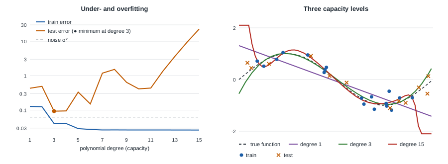
What you should see:

• train error goes down as degree increases, then settles around 0.026, below the noise $\sigma^2 = 0.0625$ : the model fits the points better than the true function itself, i.e. it learns the noise;
• test error draws a U: lowest at degree 3 (around 0.09), it then climbs back up to over 20 at degree 15 (hence the log scale);
• degree 1 misses the shape (bias), degree 15 wiggles between points and shoots off at the edges (variance);
• even at best, test error never goes below $\sigma^2$ : that’s the irreducible noise.

Measuring bias and variance directly

We apply the definition literally: retrain each model on 200 different datasets.

import numpy as np
from sklearn.pipeline import make_pipeline
from sklearn.preprocessing import PolynomialFeatures, StandardScaler
from sklearn.linear_model import LinearRegression

rng = np.random.default_rng(0)

def true_f(x):
    return np.sin(2 * np.pi * x)

def polynomial(degree):
    return make_pipeline(
        PolynomialFeatures(degree, include_bias=False),
        StandardScaler(),
        LinearRegression(),
    )

x_eval = np.linspace(0.05, 0.95, 50).reshape(-1, 1)

def bias_variance(degree, n_sets=200, n=30, noise=0.25):
    preds = np.empty((n_sets, len(x_eval)))
    for k in range(n_sets):
        xs = rng.uniform(0, 1, n)
        ys = true_f(xs) + rng.normal(0, noise, n)
        preds[k] = polynomial(degree).fit(xs.reshape(-1, 1), ys).predict(x_eval)
    mean_pred = preds.mean(axis=0)
    bias2 = np.mean((mean_pred - true_f(x_eval.ravel())) ** 2)
    variance = np.mean(preds.var(axis=0))
    return bias2, variance

print(f"{'degree':>6} | {'bias²':>8} | {'variance':>8} | {'sum':>8}")
for d in (1, 3, 5, 9, 12):
    b2, v = bias_variance(d)
    print(f"{d:>6} | {b2:8.4f} | {v:8.4f} | {b2 + v:8.4f}")

Degree	Bias²	Variance
1	0.157	0.019
3	0.003	0.009
5	0.0002	0.017
9	0.003	0.39
12	0.020	4.77

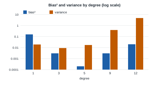
Bias² collapses from degree 3 onward, then variance explodes beyond degree 5. Their sum is smallest around degree 3: that’s the formula from section 6, checked in numbers.

---

Running project: the thesis in this framework

The thesis topic fits this framework exactly:

Element	Hot/cold prediction
Example	a DAMON memory region at time $t$
$x$	features computed from the region’s history (recency, frequency, periodicity, neighborhood…)
$y$	$1$ if the region is accessed within the next $N$ ms, $0$ otherwise
Model	logistic regression → LightGBM → LSTM
Loss	log-loss, with an asymmetric cost: a false cold (region compressed then read again) costs more than a false hot
Generalization	on the rest of the trace (the future) and on another workload

Two key differences from the toy example:

1. examples are not independent: two consecutive instants of the same region look alike. A random split becomes leakage (part 14);
2. the right metric is neither MSE nor accuracy, but a precision/recall trade-off that accounts for the cost of false colds (part 15).

---

Hands-on exercise

1. More data. Rerun the first script with n = 200, then n = 1000. Does the best degree change? Does the train/test gap at degree 15 shrink? Explain why with the bias/variance trade-off.
2. More noise. Go back to n = 30 and set noise to 0.6. What happens to the best degree? Why does a simpler model become preferable?
3. Regularization, a sneak peek. Replace LinearRegression() with Ridge(alpha=1e-3) (import from sklearn.linear_model) and keep degree 15. Compare the test error. What did regularization do to the variance? (Full answer in part 16.)
4. Running project. Without code, write 5–10 lines stating your hot/cold problem: unit of example, candidate features, exact label, horizon $N$ , what “generalizing” means. Keep it: we’ll reuse it in part 14.

Hint for question 1: with more data, each model’s variance drops, so you can afford more capacity.

---

Further resources

• An Introduction to Statistical Learning (James, Witten, Hastie, Tibshirani), chapter 2, free online: the best presentation of the bias/variance trade-off.
• The Elements of Statistical Learning, chapter 7: the more mathematical take on model selection.
• scikit-learn docs, example Underfitting vs. Overfitting.
• On this blog: scikit-learn: the full lifecycle of a model.

---

What you should be able to do before moving on

• State a supervised problem in four parts: data, model, loss, optimization
• Explain the difference between empirical and true risk, and why we need a test set
• Recognize under- and overfitting from train/test curves
• Explain the bias/variance trade-off in your own words, without formulas
• Have written the supervised framing of your hot/cold problem

Next part: Preparing data without leakage, where we generate the first simulated memory traces and see why this article’s random split would be a mistake on that data.