October 26, 2026 · 23 min read

Unsupervised learning: exploring without labels

Access profiles, PCA, k-means, DBSCAN and the pitfalls of t-SNE: recovering families of memory regions without labels, and spotting a never-seen behavior before the model gets it wrong.

Mastering AI · Technical phase · Week 2 · Part 20

Goal of this step

In part 19, we found why the model fails on the analytics workload: regions doing a scan, a behavior it had never seen. But we cheated: we knew each region’s true kind, because we had simulated it. On real DAMON traces, nobody will hand you that column.

This article’s question: can we recover these families of behaviors from the traces alone, without any label? And, better: can we see a new behavior coming before the supervised model gets it wrong?

By the end of this article you’ll be able to:

summarize a region with an access profile and pick a distance that makes sense;
apply and interpret a PCA (explained variance, loadings);
run k-means, choose $k$ without labels (elbow, silhouette), and evaluate a clustering when, for once, you have the ground truth;
know what hierarchical clustering and DBSCAN bring;
read a t-SNE plot without making it say what it doesn’t;
use all of this to detect a behavior absent from the training data.

Key concepts

1. Without labels, everything rests on the distance

Intuition. Clustering groups what looks alike. “Looking alike” means “being close”, so everything depends on the rule that measures closeness. Change the rule, you change the groups.

We’ll use the Euclidean distance from Required Maths M1, $\lVert x - x' \rVert_2$ . It has a flaw: it adds up the gaps on every column, so a column expressed on a large scale crushes the others. Hence standardization before any clustering:

z_j = \frac{x_j - \mu_j}{\sigma_j}

Each column then has zero mean and unit standard deviation: they weigh the same in the distance. That isn’t neutral, though: it’s a choice (“every column counts as much”), and the choice of the columns themselves matters even more. The code example measures what forgetting standardization costs.

Second decision: what to group. The rows of the dataset from parts 14 to 19 (one region at one instant) are too local: at a given instant, a periodic region between two activations looks like a cold one. So we group windows: one region over 700 aggregations, summarized in a few numbers (its profile).

2. PCA: looking at the data from the right angle

Intuition. Six columns means six dimensions: impossible to draw. PCA looks for the plane on which the shadow of the point cloud is most spread out, so the one that loses the least information.

You saw the mechanics in Required Maths M3: the principal axes are the eigenvectors of the covariance matrix of the standardized data, and the share of variance carried by axis $j$ is

\frac{\lambda_j}{\lambda_1 + \dots + \lambda_p}

Two readings:

the explained variance tells you how many axes are enough (if PC1 + PC2 carry 90%, the 2D drawing is faithful);
the loadings (the coordinates of the eigenvectors) tell you what each axis measures. An axis where all the intensity columns have a strong positive loading is an “activity” axis.

Careful: the sign of an axis is arbitrary (an eigenvector and its opposite both work), and PCA only sees linear relationships.

3. k-means: $k$ centers, and each point goes to the nearest

Intuition. Place $k$ centers at random. Each point joins the nearest center; each center moves to the middle of its points; repeat until nothing moves.

It’s a descent on the inertia, the sum of squared distances from each point to its center:

\min_{c_1, \dots, c_k} \; \sum_{i=1}^{n} \min_{j \in \{1,\dots,k\}} \lVert x_i - c_j \rVert_2^2

The problem isn’t convex (M6): the result depends on the initialization, hence n_init=10 (ten starts, keep the best). And k-means assumes round groups of comparable sizes: it would rather split a large spread-out group in two than isolate a small compact one.

Choosing $k$ without labels. Inertia always drops as $k$ grows: you look for an elbow, often blurry. The silhouette is sharper. For a point $i$ , with $a_i$ its mean distance to the points of its own cluster and $b_i$ its mean distance to the points of the nearest other cluster:

s_i = \frac{b_i - a_i}{\max(a_i, b_i)}

$s_i$ close to 1: the point is at home. Close to 0: it sits on the border. Negative: it would be better off elsewhere. Take the $k$ that maximizes the mean silhouette.

Evaluating when you have the truth. Here, for once, we know the kinds (simulated). The ARI (adjusted Rand index) measures the agreement between two partitions, regardless of cluster numbers: 1 = identical, 0 = no better than chance. We use it only as a check, never to choose: on real traces, it won’t exist.

4. Two other families: hierarchical and density-based

Hierarchical clustering (Ward). Start with one cluster per point and, at each step, merge the two clusters whose union increases the inertia the least. You get a tree of merges (dendrogram) that you cut at the level you want. Upside: no random initialization, and every value of $k$ at once.
DBSCAN. A cluster is a dense area: a point is a “core” point if it has at least min_samples neighbors within eps, and neighboring core points chain together. Isolated points are labeled noise ( $-1$ ). Upsides: no $k$ to choose, arbitrary shapes. Trade-off: eps to tune. A heuristic: plot each point’s distance to its min_samples-th neighbor, and take eps near the elbow of that curve.

5. t-SNE and UMAP: made for looking, not for measuring

Intuition. t-SNE places points in 2D so that close neighbors stay neighbors. It does that very well, at the expense of everything else.

What t-SNE (and UMAP, built on the same idea) does not preserve:

group sizes: t-SNE inflates dense areas and shrinks diffuse ones;
distances between groups: two groups far apart on the plot aren’t necessarily far apart in the data;
the absence of structure: on pure noise, it happily draws clumps.

The result also depends on the perplexity (roughly, how many neighbors are taken into account) and on the seed. The rule: t-SNE is for forming hypotheses to be checked afterwards in the original space, never for proving them. Never cluster on t-SNE coordinates.

Code example

As in parts 15 to 19, we take the script from part 14 as is, then append the four blocks below. The two workloads are those of parts 18 and 19: jvm (70% periodic regions) and analytics (which contains the scans). The whole thing runs in about ten seconds (numpy 2.5, pandas 3.0, scikit-learn 1.9, scipy 1.18).

Access profiles, then a PCA

Each region is cut into four windows of 700 aggregations, aligned on the regime change ( $t = 2100$ ) so that a window never mixes two kinds. Each window is summarized in six numbers, computed without any label:

Column	What it measures
`log_intensity`	mean number of accesses per aggregation (log)
`frac_active`	share of aggregations with at least one access
`log_burst_len`	mean length of an activity period (log)
`log_gap`	mean gap between two activity starts (log)
`irregularity`	standard deviation / mean of those gaps: 0 = metronome
`acf_peak`	highest autocorrelation peak between lags 5 and 299: 1 = perfectly periodic

Autocorrelation is the correlation of the series with a shifted copy of itself (M7): it’s the rigorous version of the “periodicity” announced in part 14. The logs bring very skewed quantities (from 0.01 to 4 accesses per aggregation) onto a scale where distances make sense.

# Continuation of the part 14 script: T, N_REGIONS, BLOCK_SIZE, T_CHANGE, KINDS,
# simulate_segment, np and pd are already defined.
from sklearn.preprocessing import StandardScaler
from sklearn.decomposition import PCA


def simulate_workload(seed, kinds, p, scan_cycle=240):
    """Part 19's simulate_workload: same traces, plus each region's true kind."""
    r = np.random.default_rng(seed)
    accesses = np.zeros((N_REGIONS, T), dtype=int)
    kind_of = np.empty((N_REGIONS, 2), dtype=object)
    times = np.arange(T)
    for block in range(N_REGIONS // BLOCK_SIZE):
        before = r.choice(kinds, p=p)
        after = r.choice(kinds, p=p) if r.random() < 0.4 else before
        for reg in range(block * BLOCK_SIZE, (block + 1) * BLOCK_SIZE):
            kind_of[reg] = before, after
            for start, end, kind in [(0, T_CHANGE, before), (T_CHANGE, T, after)]:
                if kind == "scan":
                    active = (times[start:end] - 2 * reg) % scan_cycle < 2
                    accesses[reg, start:end] = active * r.poisson(6, end - start)
                else:
                    accesses[reg, start:end] = simulate_segment(kind, end - start, r)
    return accesses, kind_of


def profile(a):
    """Summary of one access window in 6 numbers, without any label."""
    active = (a > 0).astype(int)
    starts = np.flatnonzero(np.diff(np.r_[0, active]) == 1)        # activity starts
    ends = np.flatnonzero(np.diff(np.r_[active, 0]) == -1)         # activity ends
    gaps = np.diff(starts)
    x = active - active.mean()
    acf = np.array([x[:-k] @ x[k:] for k in range(5, 300)]) / max(x @ x, 1e-9)
    return {
        "log_intensity": np.log1p(a.mean()),                         # mean accesses per aggregation
        "frac_active": active.mean(),                                # share of time active
        "log_burst_len": np.log1p((ends - starts + 1).mean()) if len(starts) else 0.0,
        "log_gap": np.log1p(gaps.mean()) if len(gaps) else np.log1p(len(a)),
        "irregularity": gaps.std() / gaps.mean() if len(gaps) > 1 else 1.0,
        "acf_peak": acf.max(),                                       # 1 = perfectly periodic
    }


# Windows of 700 aggregations, aligned on the regime change (t = 2100)
WINDOWS = [(0, 700), (700, 1400), (1400, 2100), (2100, 2800)]
rows = []
for name, (acc, kinds) in {"jvm": simulate_workload(11, KINDS, [0.7, 0.1, 0.1, 0.1]),
                           "analytics": simulate_workload(12, KINDS + ["scan"],
                                                          [0.1, 0.15, 0.25, 0.1, 0.4])}.items():
    for reg in range(N_REGIONS):
        for start, end in WINDOWS:
            rows.append({**profile(acc[reg, start:end]), "workload": name, "region": reg,
                         "start": start, "kind": kinds[reg, int(start >= T_CHANGE)]})
profiles = pd.DataFrame(rows)
COLS = ["log_intensity", "frac_active", "log_burst_len", "log_gap", "irregularity", "acf_peak"]
pd.set_option("display.width", 120)
pd.set_option("display.max_columns", 20)
print(profiles.shape, {str(k): int(v) for k, v in profiles.kind.value_counts().items()})
print(profiles.groupby("kind")[COLS].median().round(2))

# PCA on the standardized profiles
Z = StandardScaler().fit_transform(profiles[COLS])
pca = PCA().fit(Z)
print("explained variance:", pca.explained_variance_ratio_.round(3),
      "| cumulative PC1+PC2:", pca.explained_variance_ratio_[:2].sum().round(3))
print(pd.DataFrame(pca.components_[:2].T, index=COLS, columns=["PC1", "PC2"]).round(2))

Output: 768 windows (2 workloads × 96 regions × 4 windows): 304 periodic, 208 hot, 136 scan, 100 cold and 20 bursty. The medians per kind, which the clustering will never see:

Kind	`log_intensity`	`frac_active`	`log_burst_len`	`log_gap`	`irregularity`	`acf_peak`
bursty	0.47	0.12	2.04	3.94	0.83	0.39
cold	0.01	0.01	0.69	4.47	0.71	0.16
hot	1.30	0.93	2.67	2.72	0.83	0.11
periodic	0.38	0.07	1.39	3.69	0.00	0.94
scan	0.05	0.01	1.10	5.48	0.00	0.67

The signatures are clear: hot regions are active 93% of the time; periodic and scan regions are metronomes (zero irregularity), but the scan comes back far less often (a gap of $e^{5.48} - 1 \approx 240$ aggregations versus $e^{3.69} - 1 \approx 40$ ); cold and bursty regions are irregular, bursty ones being much more intense.

PCA. The first two axes carry 69.8% and 18.6% of the variance, i.e. 88.4%: the 2D drawing will be faithful. The loadings:

Column	PC1	PC2
`log_intensity`	0.46	0.31
`frac_active`	0.48	0.08
`log_burst_len`	0.42	0.22
`log_gap`	−0.33	−0.45
`irregularity`	0.39	−0.51
`acf_peak`	−0.36	0.62

PC1 is an “activity” axis: intensity, active share and burst length push in the same direction, the gap between activations in the other. Hot regions are on the far right.
PC2 is a “regularity” axis: strong autocorrelation at the top, irregularity at the bottom. Periodic regions are at the top, cold ones at the bottom.

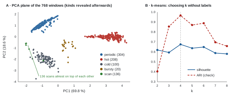
Two panels. A: PCA plane (PC1 69.8%, PC2 18.6%) of the 768 access-profile windows, colored afterwards by their true kind; periodic, hot, cold, bursty and scan regions form separate groups, the 136 scans almost on top of each other. B: k-means silhouette and ARI for k from 2 to 8; silhouette peaks at k = 4 (0.676), where ARI is 0.966.

In panel A, the colors are added afterwards: the PCA never saw them. Five separate groups show up anyway. The 136 scans almost fit in a single point: the same mechanism (2 active aggregations every 240) gives almost the same profile from one region to the next.

k-means, Ward, DBSCAN

from sklearn.cluster import KMeans, AgglomerativeClustering, DBSCAN
from sklearn.neighbors import NearestNeighbors
from sklearn.metrics import silhouette_score, adjusted_rand_score

# Choosing k without labels: inertia (elbow) and silhouette. ARI uses the hidden kinds: a check only.
for k in range(2, 9):
    km = KMeans(n_clusters=k, n_init=10, random_state=0).fit(Z)
    print(f"k = {k} | inertia {km.inertia_:7.1f} | silhouette {silhouette_score(Z, km.labels_):.3f}"
          f" | ARI {adjusted_rand_score(profiles.kind, km.labels_):.3f}")

for k in (4, 6):
    km = KMeans(n_clusters=k, n_init=10, random_state=0).fit(Z)
    print(f"\nk-means, k = {k}\n", pd.crosstab(km.labels_, profiles.kind))

# Same thing without standardizing: distances are dominated by the large-scale columns
raw = KMeans(n_clusters=4, n_init=10, random_state=0).fit(profiles[COLS])
print("\nraw standard deviations:", profiles[COLS].std().round(2).to_dict())
print("k-means k = 4 without standardizing: ARI", round(adjusted_rand_score(profiles.kind, raw.labels_), 3))
print(pd.crosstab(raw.labels_, profiles.kind))

# Two other families: hierarchical (Ward) and density-based (DBSCAN)
ward = AgglomerativeClustering(n_clusters=4, linkage="ward").fit(Z)
print("\nWard, 4 clusters: ARI", round(adjusted_rand_score(profiles.kind, ward.labels_), 3))
d10 = NearestNeighbors(n_neighbors=10).fit(Z).kneighbors(Z)[0][:, -1]   # distance to the 10th neighbor
print("distance to the 10th neighbor, 50/90/99% quantiles:", np.quantile(d10, [0.5, 0.9, 0.99]).round(2))
for eps in (0.5, 0.8):
    db = DBSCAN(eps=eps, min_samples=10).fit(Z)
    print(f"\nDBSCAN eps = {eps}: ARI {adjusted_rand_score(profiles.kind, db.labels_):.3f} (-1 = noise)\n",
          pd.crosstab(db.labels_, profiles.kind))

Choosing $k$ .

$k$	Inertia	Silhouette	ARI (check)
2	1,674.4	0.620	0.404
3	964.7	0.595	0.855
4	598.2	0.676	0.966
5	382.9	0.638	0.870
6	312.1	0.649	0.889
7	250.8	0.589	0.697
8	194.9	0.581	0.659

Inertia drops with no clear elbow; the silhouette, on the other hand, points to $k = 4$ , and that’s exactly where the ARI (computed with the hidden kinds) is best: 0.966. The label-free criterion found the right setting. But there are five kinds, not four. The clusters:

Cluster ( $k = 4$ )	bursty	cold	hot	periodic	scan
0	0	0	208	0	0
1	0	5	0	0	132
2	0	0	0	304	0
3	20	95	0	0	4

The 20 bursty windows are swallowed by the cold ones. They’re only 20 windows out of 768: separating them barely reduces the inertia.
With $k = 5$ , k-means still doesn’t isolate them: it splits the hot regions in two (106 + 102), because a large spread-out group costs more inertia than a small group off to the side. It takes $k = 6$ to get a cluster of 20 pure bursty windows. That’s the “round groups of comparable sizes” bias from section 3, with numbers.
The 4 scans classified as cold are regions 88 to 91 on a window where they’re activated only twice: a single gap between two starts, so an irregularity that can’t be measured (the code then sets it to 1.0). A window that’s too short compared to the cycle makes a behavior indistinguishable: exercise 1 pushes this effect all the way.

Without standardizing, the ARI at $k = 4$ drops to 0.746: scans and cold regions merge (136 + 98), hot regions are split in two (108 + 100), and bursty windows join the periodic ones. The raw standard deviations range from 0.37 (acf_peak) to 1.04 (log_gap): the raw distance is mostly made of intensity and gap between activations, two columns where scans and cold regions look alike (few accesses, long silences). What sets them apart, regularity, weighs too little.

Ward (4 clusters) does barely better than k-means: ARI 0.975, with the same confusion of the bursty windows.

DBSCAN. The distance to the 10th neighbor is 0.17 at the median, 0.47 at the 90% quantile and 1.11 at the 99% quantile: we try eps = 0.5 (near the elbow) and 0.8.

	`eps` = 0.5	`eps` = 0.8
Clusters	4	5
Noise points	38, including all 20 bursty	5
Bursty windows	all noise	18 in their own cluster
ARI	0.972	0.988

With eps = 0.5, DBSCAN says something interesting: bursty windows don’t form a dense enough area, they’re anomalies. With eps = 0.8, it recovers all five kinds, without being given any $k$ . Both readings are true; it’s up to you to decide whether 20 windows make a family or an exception.

The pitfalls of t-SNE, measured

from sklearn.manifold import TSNE
from scipy.spatial.distance import pdist


def spread(E, kind):
    """Mean distance between two points of the same kind."""
    return pdist(E[(profiles.kind == kind).values]).mean()


# Do the relative sizes of the groups survive t-SNE?
for name, E in [("standardized profiles", Z)] + [
        (f"t-SNE perplexity {p}", TSNE(perplexity=p, random_state=0).fit_transform(Z)) for p in (5, 30, 100)]:
    s = {k: spread(E, k) for k in ("hot", "periodic", "scan")}
    print(f"{name:>22} | hot {s['hot']:6.2f} | periodic {s['periodic']:6.2f} | "
          f"scan {s['scan']:6.2f} | hot / periodic {s['hot'] / s['periodic']:.2f}")

# And on pure noise, with no structure at all?
noise = np.random.default_rng(0).normal(size=Z.shape)
E = TSNE(perplexity=30, random_state=0).fit_transform(noise)
for name, X in [("raw noise", noise), ("t-SNE of noise", E)]:
    print(f"{name:>15} | k-means k = 4 silhouette: "
          f"{silhouette_score(X, KMeans(n_clusters=4, n_init=10, random_state=0).fit_predict(X)):.3f}")

Mean distance between two windows of the same kind:

Representation	hot	periodic	scan	hot / periodic
Standardized profiles (the truth)	1.53	0.75	0.18	2.05
t-SNE, perplexity 5	38.02	54.60	63.33	0.70
t-SNE, perplexity 30	13.52	18.50	12.01	0.73
t-SNE, perplexity 100	3.49	4.38	2.44	0.80

t-SNE inverts sizes. In the data, hot regions are twice as spread out as periodic ones; on every t-SNE plot, they look more compact.
The tightest group can become the widest. The scans almost fit in a single point (0.18), but with a perplexity of 5, t-SNE makes them the most spread-out group (63.33): it stretches near-identical points to give them room.
t-SNE invents groups. On 768 points of pure Gaussian noise, the silhouette of a 4-cluster k-means is 0.110 in the original space (no structure) and 0.381 on the t-SNE coordinates: the plot suggests groups that don’t exist.

Remember it for the thesis: a t-SNE plot is an illustration, never a result.

Spotting, without labels, a behavior never seen before

This is the direct link with parts 18 and 19: the supervised model trained without the analytics workload failed on the scans. Can we see, without any label, that the analytics windows contain something jvm never showed?

# Running project: spotting, without any label, a behavior absent from the training data
km = KMeans(n_clusters=6, n_init=10, random_state=0).fit(Z)
print(pd.crosstab(km.labels_, profiles.workload))             # a cluster with no jvm window at all?

jvm, ana = profiles[profiles.workload == "jvm"], profiles[profiles.workload == "analytics"]
scaler = StandardScaler().fit(jvm[COLS])                     # everything is fitted on jvm only
Zj, Za = scaler.transform(jvm[COLS]), scaler.transform(ana[COLS])

# a) distance to the nearest jvm centroid (k chosen by silhouette on jvm)
k_jvm = max(range(2, 9), key=lambda k: silhouette_score(
    Zj, KMeans(n_clusters=k, n_init=10, random_state=0).fit_predict(Zj)))
km_jvm = KMeans(n_clusters=k_jvm, n_init=10, random_state=0).fit(Zj)
d_centroid_j, d_centroid_a = km_jvm.transform(Zj).min(1), km_jvm.transform(Za).min(1)

# b) mean distance to the 5 nearest jvm windows (local density)
nn = NearestNeighbors(n_neighbors=5).fit(Zj)
d_knn_j = nn.kneighbors(Zj, n_neighbors=6)[0][:, 1:].mean(1)  # exclude the point itself
d_knn_a = nn.kneighbors(Za)[0].mean(1)

# Threshold: 99% of jvm windows are below it; flag the analytics windows above it
res = ana.assign(centroid=d_centroid_a > np.quantile(d_centroid_j, 0.99),
                 knn=d_knn_a > np.quantile(d_knn_j, 0.99)).groupby("kind")
print(f"k chosen on jvm: {k_jvm}")
print(pd.DataFrame({"windows": res.size(), "flagged (centroid)": res.centroid.mean(),
                    "flagged (5 neighbors)": res.knn.mean()}).round(2))

First reading: cluster composition. With $k = 6$ on both workloads, two clusters contain (almost) no jvm window: one has 134 analytics windows for 2 jvm (the scans), the other 20 analytics for 0 jvm (the bursty ones). A cluster that exists only in the new data is a warning sign.

Second reading: a distance to the known. We fit everything on jvm only, and flag an analytics window if it’s farther from jvm than 99% of the jvm windows themselves.

Kind (analytics)	Windows	Flagged (distance to centroid)	Flagged (5 nearest neighbors)
bursty	20	0.05	1.00
cold	44	0.00	0.02
hot	148	0.03	0.01
periodic	36	0.00	0.00
scan	136	0.00	1.00

The distance to the centroid fails completely: not a single scan flagged. The silhouette chooses $k = 3$ on jvm, and the hot cluster is very spread out: the 99% threshold is therefore wide, and the scans, foreign as they are, slip under it. The “round groups” assumption of k-means again.
The distance to the 5 nearest neighbors succeeds: 100% of scans and bursty windows flagged, 0 to 2% false alarms on known behaviors. It measures local density: a window is “new” if it has no close jvm neighbor, whatever the shape of the groups.

So we have a detector, trained without a single label, that would have raised its hand on exactly the two behaviors jvm had never shown, before the supervised model even got anything wrong.

Running project: what this changes for the thesis

Chapter 4 (exploratory analysis) has a method. Window profiles, standardization, PCA for explained variance and loadings, k-means with silhouette, then a check with Ward and DBSCAN. If three families of algorithms agree, the structure is probably real.
H1 can also be tested without labels. The regularity columns (irregularity, acf_peak) carry PC2 and separate periodic from cold regions. Exercise 2 shows that with only the intensity columns, the ARI collapses. On real traces, if PC2 remains a “regularity” axis, that’s an argument for periodicity, independent of any model.
You now have slices for error analysis. Part 19 asked which slices to use without a “true kind” (exercise 5). Answer: the profile clusters. Compute the excess loss per cluster instead of per kind.
A safeguard for the daemon. The distance to the $k$ nearest training windows is a cheap drift (out-of-distribution) detector. If the share of flagged windows exceeds a threshold, the daemon can fall back to a cautious policy (stop compressing) instead of trusting a model outside its domain. We’ll come back to this in part 28 (monitoring).
Watch causality if you use it online. Here, the profiles look at whole windows, which is legitimate for exploration. As a feature of a prediction model, a profile must be computed on the past 700 aggregations, otherwise it’s part 14’s leak from the future.
t-SNE in the thesis: in an appendix, as an illustration, with the perplexity stated, and never as proof of a separation.

Hands-on exercise

Window size. Replace WINDOWS with nine windows of 300 aggregations (from 0 to 2,700) and rerun the choice of $k$ . Which $k$ does the silhouette pick? What happens to the scans? Relate your answer to the cycle length (240 aggregations).
Without regularity. Redo the k-means keeping only log_intensity, frac_active and log_burst_len. Which $k$ does the silhouette pick, and what ARI do you get at $k = 4$ ? Which kinds merge? What does that say about hypothesis H1?
Why the centroid fails. Print the 99% threshold of the distance to the jvm centroid and the median distance of the scan windows. Then print the crosstab of the 3 jvm clusters against the jvm kinds. Which cluster makes the threshold so wide?
A Gaussian mixture. Replace k-means with GaussianMixture(k, covariance_type="full", random_state=0, n_init=3) for $k$ from 2 to 8, and choose $k$ with the BIC criterion (.bic(Z), lowest is best). Which $k$ do you get? Why does the BIC keep dropping? (Think of the 136 scans almost on top of each other.)
Running project. On your real DAMON traces, compute the window profiles per region, run the PCA and give an interpretation of PC1 and PC2 from the loadings. Then compute the excess loss of your part 19 model per profile cluster.

Hints. Question 1: 1,728 windows; the silhouette picks $k = 3$ (0.655), ARI 0.84; the 304 scan windows land with 215 cold ones: with 300 aggregations, a window often contains only one or two activations, and irregularity can no longer be measured. Question 2: the silhouette picks $k = 2$ (ARI 0.378); at $k = 4$ , the ARI is 0.47, and the 136 scans, the 100 cold windows and 77 periodic ones share a cluster: without the regularity columns, a slow metronome looks like silence. Question 3: threshold 3.02, median scan distance 2.78; the cluster of the 60 jvm hot windows is the most spread out. Question 4: the BIC keeps dropping up to $k = 8$ (from −700.4 to −15,856.8); at $k = 4$ the ARI is 0.973. Near-identical points allow an almost zero covariance, hence an exploding likelihood: the BIC isn’t reliable on such degenerate data.

Further resources

James, Witten, Hastie and Tibshirani, An Introduction to Statistical Learning (ISLR), chapter 12: PCA, k-means and hierarchical clustering.
scikit-learn docs: Clustering (comparison of algorithms and metrics, including silhouette and ARI) and Decomposition (PCA).
Ester et al., A Density-Based Algorithm for Discovering Clusters in Large Spatial Databases with Noise (KDD 1996): the DBSCAN paper.
Wattenberg, Viégas and Johnson, How to Use t-SNE Effectively (Distill, 2016): the pitfalls of t-SNE, with interactive examples.
Refreshers: M1 · Vectors, dot product and norms for distances, M3 · Eigenvalues, SVD and PCA for PCA.

What you should be able to do before moving on

Explain why we standardize before clustering, and measure what forgetting it costs
Build a label-free window profile and justify the choice of columns
Apply a PCA, read the explained variance and interpret the loadings of the first axes
Run k-means, choose $k$ with the silhouette, and know its bias toward round groups of comparable sizes
Evaluate a clustering with the ARI when a ground truth exists, without using it to choose
Tune DBSCAN’s eps with the distance to the k-th neighbor, and interpret noise points
Name three things a t-SNE plot does not preserve
Build a new-behavior detector based on distance to nearest neighbors

Next part: A neural network by hand with PyTorch (part 21). We leave trees behind: we rebuild in PyTorch the small network written in NumPy in the M12 wrap-up, with autograd, nn.Module and a real training loop, before moving on to sequence models.