October 23, 2026 · 17 min read

Serious validation and tuning

Time-based folds with purge, grid vs random vs Optuna, and leave-one-workload-out: tuning models without fooling yourself, and measuring the cost of an unseen workload.

Mastering AI · Technical phase · Week 2 · Part 18

Goal of this step

Since part 15, we’ve chosen everything (threshold, features, model size) on a single validation period, $1400 \le t < 1790$ . Part 17 showed the limit: models that are almost identical in validation give test costs between 0.637 and 0.826. A single period is a single measurement, so a single draw of the noise.

By the end of this article you’ll be able to:

explain why shuffled K-fold is forbidden on time-ordered traces, with numbers;
build a time-based cross-validation with purge and read the spread of its folds;
compare grid, random search and Optuna at equal budget, without over-reading the winner;
set up a leave-one-workload-out to test generalization to a workload never seen before.

Key concepts

1. Why shuffled K-fold is forbidden here

Intuition. Classic K-fold splits the rows at random into $K$ chunks, trains on $K-1$ and validates on the last one. On our traces, two rows that are neighbors in time are almost identical: shuffling puts row $t$ in training and row $t+1$ in validation. That’s the leak through the split from part 14, repeated $K$ times.

K-fold assumes independent, identically distributed examples (the framework of part 13). Ours are neither: they’re correlated in time, and the distribution changes in the middle of the trace.

2. Time-based cross-validation

Intuition. We replay the production situation several times, “train on the past, predict what comes next”, moving the cut date forward.

We split the development period into $K + 1$ consecutive blocks. Fold $i$ trains on blocks $0$ to $i - 1$ and validates on block $i$ :

\text{train}_i = \{\, t < b_i - H \,\} \qquad \text{val}_i = \{\, b_i \le t < b_{i+1} - H \,\}

The purge of $H$ aggregations before each validation comes from part 14: a training label looks $H$ steps ahead, so it must not see the validation. The second purge (at the end of each validation block except the last) keeps validation labels from looking into the next block.
Expanding window: each fold keeps the whole past. Rolling window: we only keep the last $w$ blocks, useful when the old past no longer looks like the present.
scikit-learn’s TimeSeriesSplit does the same thing, with a gap parameter for the purge, but it splits row numbers, assuming one row per time step. We have 96 rows per time step (one per region), so we split on t directly, in ten lines of code.

3. A validation score is a random variable

Intuition. Each fold gives a slightly different AUC. The mean is the estimate; the spread tells you how much to trust it.

With $K$ folds and scores $s_1, \dots, s_K$ , we report the mean $\bar{s}$ and the standard deviation across folds. To compare two settings A and B, we compare fold by fold: both see exactly the same data, so the differences $s_k^A - s_k^B$ cancel out each fold’s own difficulty. That’s the paired-sample idea from Required Maths M9.

Two caveats:

the folds are not independent (the training sets overlap), so no naive Student t-test on 4 values; we check whether the gap always has the same sign and whether it exceeds the spread across folds;
the mean over folds estimates performance under the conditions of the development period. If the test contains something new (a regime change), no internal validation can foresee it.

4. Searching hyperparameters: grid, random, Bayesian optimization

Intuition. Each trial costs $K$ trainings. The question is: where do you spend a fixed budget of trials?

Grid: every combination of a few values per parameter. Simple, but with 4 parameters and 3 values that’s already 81 trials, and each parameter is only tried at 3 values.
Random search: draw each parameter at random within a range. At equal budget, each parameter is tried at as many values as there are trials. When only one or two parameters really matter, this is clearly better than a grid (Bergstra and Bengio, 2012).
Bayesian optimization (Optuna, TPE): after a few random trials, the algorithm splits trials into “good” and “bad”, models the two parameter distributions $\ell(x)$ and $g(x)$ , and proposes the point that maximizes $\ell(x) / g(x)$ : where good trials are frequent and bad ones rare.

For “multiplicative” parameters (learning rate, number of leaves, min_child_samples), we sample on a log scale: going from 0.01 to 0.02 matters as much as going from 0.1 to 0.2.

5. Overfitting the validation

Intuition. If you run 100 trials whose scores only differ by noise, the best one will still come out on top, by luck. Its score is biased upward: that’s the winner’s curse.

The more trials you run on the same validation, the more it becomes part of training. The remedies:

a test looked at only once, after all choices (part 14);
nested cross-validation: an inner loop picks the hyperparameters, an outer loop measures the performance of the whole selection procedure;
distrust any gap smaller than the spread across folds.

6. Leave-one-group-out: generalizing to an unseen workload

Intuition. Your daemon will run on programs you never traced. The real question isn’t “does it predict the rest of this trace well?” but “does it predict a trace from another program well?”.

We group the data by workload (a program, a load). For each workload $g$ , we train on all the others and test on $g$ . Combined with the time-based split, this gives three protocols, tested on exactly the same rows (the end of $g$ ’s trace):

Protocol	Training	What it measures
In-workload	the past of $g$	predicting the rest of a known workload
Leave-one-workload-out	the past of the other workloads	generalizing to an unseen workload
All	the past of all of them, $g$ included	what having already seen $g$ brings

The gap between “in-workload” and “leave-one-workload-out” is the price of novelty.

Code example

As in parts 15 to 17, we reuse the part 14 script as is, then add the three blocks below after it, in the same file. The development period is $t < 1790$ (the train and validation of the previous parts combined), the test stays $t \ge 1800$ . The whole thing runs in about three minutes (numpy 2.5, pandas 3.0, scikit-learn 1.9, lightgbm 4.7, optuna 5.0).

Shuffled K-fold versus time-based folds

# Continuation of the part 14 script: df, FEATURES, H, T, np, pd, roc_auc_score,
# simulate_segment, build_dataset, KINDS, BLOCK_SIZE, N_REGIONS and T_CHANGE are already defined.
import itertools
import time
import lightgbm as lgb
import optuna
from sklearn.model_selection import KFold

# Development = everything before the test (train + validation of parts 15 to 17)
t_test = 1800
dev = df[df.t < t_test - H].reset_index(drop=True)
test = df[df.t >= t_test]


# 1. Shuffled K-fold versus time-based folds with purge
def time_folds(d, k=4, purge=H):
    """Expanding window: train on the past, validate on the next block."""
    bounds = np.linspace(d.t.min(), d.t.max() + 1, k + 2).astype(int)
    for i in range(1, k + 1):
        tr = np.flatnonzero(d.t < bounds[i] - purge)              # purge before validation
        end = bounds[i + 1] - purge if i < k else bounds[i + 1]   # labels don't overlap the next block
        va = np.flatnonzero((d.t >= bounds[i]) & (d.t < end))
        yield tr, va


def cv_score(params, d, splits):
    scores = []
    for tr, va in splits:
        m = lgb.LGBMClassifier(**params, random_state=0, verbose=-1).fit(d.iloc[tr][FEATURES], d.y.iloc[tr])
        scores.append(roc_auc_score(d.y.iloc[va], m.predict_proba(d.iloc[va][FEATURES])[:, 1]))
    return np.array(scores)


BASE = dict(num_leaves=31, n_estimators=100, learning_rate=0.1)
print("block bounds:", np.linspace(dev.t.min(), dev.t.max() + 1, 6).astype(int))
shuffled = cv_score(BASE, dev, KFold(4, shuffle=True, random_state=0).split(dev))
timewise = cv_score(BASE, dev, list(time_folds(dev)))
m = lgb.LGBMClassifier(**BASE, random_state=0, verbose=-1).fit(dev[FEATURES], dev.y)
print(f"shuffled K-fold {shuffled.round(3)} mean {shuffled.mean():.3f}")
print(f"time folds {timewise.round(3)} mean {timewise.mean():.3f} std {timewise.std(ddof=1):.3f}")
print(f"test (only once) {roc_auc_score(test.y, m.predict_proba(test[FEATURES])[:, 1]):.3f}")

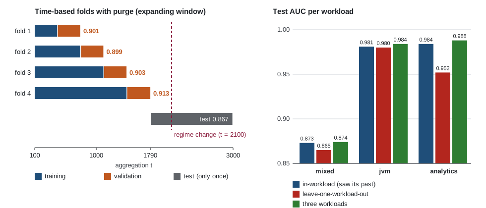
The blocks start at $t$ = 100, 438, 776, 1,114 and 1,452; the last one ends at 1,790.

Protocol	AUC per fold	Mean
Shuffled K-fold	0.937 · 0.939 · 0.940 · 0.940	0.939
Time-based folds with purge	0.901 · 0.899 · 0.903 · 0.913	0.904 (std 0.006)
Test, looked at only once		0.867

Shuffled K-fold lies by 3.5 points on the same period with the same model. Its four folds are almost identical (0.937 to 0.940): the low spread isn’t reassuring, it confirms we keep measuring the same leak.
Time-based folds are honest, but not clairvoyant. They announce 0.904; the test gives 0.867. The whole development period comes before the regime change at $t = 2100$ , so no fold contains it. Time-based cross-validation estimates performance well “as long as the workload doesn’t change”, and nothing more.

Grid, random and Optuna, at equal budget

# 2. Same budget (18 trials), three ways to search
optuna.logging.set_verbosity(optuna.logging.WARNING)
FOLDS = list(time_folds(dev))
BUDGET = 18
trials = {}

# a) Grid: 3 x 3 x 2 = 18 combinations
grid = [dict(num_leaves=f, learning_rate=lr, n_estimators=n)
        for f, lr, n in itertools.product([8, 31, 127], [0.03, 0.1, 0.3], [50, 200])]
trials["grid"] = [(p, cv_score(p, dev, FOLDS)) for p in grid]

# b) Random search: 18 draws, log scale for "multiplicative" parameters
rng_r = np.random.default_rng(0)
log_unif = lambda a, b: float(np.exp(rng_r.uniform(np.log(a), np.log(b))))
random_draws = [dict(num_leaves=int(log_unif(4, 256)), learning_rate=log_unif(0.01, 0.3),
                     n_estimators=int(rng_r.integers(20, 301)), min_child_samples=int(log_unif(5, 1000)))
                for _ in range(BUDGET)]
trials["random"] = [(p, cv_score(p, dev, FOLDS)) for p in random_draws]


# c) Optuna (TPE): 6 random trials, then it proposes where things look promising
def objective(trial):
    p = dict(num_leaves=trial.suggest_int("num_leaves", 4, 256, log=True),
             learning_rate=trial.suggest_float("learning_rate", 0.01, 0.3, log=True),
             n_estimators=trial.suggest_int("n_estimators", 20, 300),
             min_child_samples=trial.suggest_int("min_child_samples", 5, 1000, log=True))
    s = cv_score(p, dev, FOLDS)
    trial.set_user_attr("folds", s.tolist())
    return s.mean()


study = optuna.create_study(direction="maximize",
                            sampler=optuna.samplers.TPESampler(seed=0, n_startup_trials=6))
study.optimize(objective, n_trials=BUDGET)
trials["optuna"] = [(t.params, np.array(t.user_attrs["folds"])) for t in study.trials]

for name, lst in trials.items():
    p, s = max(lst, key=lambda e: e[1].mean())
    m = lgb.LGBMClassifier(**p, random_state=0, verbose=-1).fit(dev[FEATURES], dev.y)
    auc_test = roc_auc_score(test.y, m.predict_proba(test[FEATURES])[:, 1])
    gaps = s - timewise                                     # fold by fold, against BASE
    print(f"{name:>6} | best CV {s.mean():.4f} | per-fold gain over BASE {gaps.round(3)} | "
          f"test {auc_test:.4f} | { {k: round(v, 3) for k, v in p.items()} }")

Reference: the base setting (31 leaves, 100 trees, rate 0.1) gets 0.904 in cross-validation and 0.867 on the test.

Method	Best setting	CV AUC	Per-fold gain over base	Test AUC
Grid	31 leaves, rate 0.03, 50 trees	0.9063	+0.002 · +0.001 · +0.002 · +0.004	0.8687
Random	56 leaves, rate 0.025, 106 trees, `min_child_samples` 5	0.9089	+0.001 · +0.004 · +0.007 · +0.008	0.8735
Optuna	40 leaves, rate 0.044, 101 trees, `min_child_samples` 37	0.9082	+0.004 · +0.001 · +0.005 · +0.006	0.8729

Tuning pays, a little. All three methods beat the base on each of the four folds: the gain is real, but it’s worth 2 to 5 thousandths of AUC. It carries over to the test (0.867 → 0.869 to 0.874).
We can’t rank the three methods. Between the best (0.9089) and the worst (0.9063), the gap is 0.003, half the standard deviation across folds (0.006), with a single seed and 18 trials. Here random search is ahead; with another seed it could be Optuna. Optuna becomes really useful when the budget is large and each trial expensive.
The grid won on an edge. Its best point uses the smallest tested value of the learning rate (0.03) and of the number of trees (50): the optimum may lie outside the grid. That’s the classic signal to widen it or switch to random search. The grid also never touched min_child_samples.
The validation–test gap (about 3.5 points) is seven times larger than anything tuning gained. The bottleneck isn’t model tuning; it’s the regime change, already at the heart of parts 16 and 17.

Leave-one-workload-out

We add two simulated workloads to the “mixed” workload of the previous parts:

jvm: 70% periodic blocks, a different mix of the same four behaviors;
analytics: 40% of blocks doing a scan, a new behavior. Region reg is read every 240 aggregations, 2 aggregations after its neighbor reg - 1, like a sequential table scan. Neither of the other two workloads contains this behavior, and 240 is far beyond the 15 to 60 periods of periodic regions.

Each workload keeps its regime change at $t = 2100$ . The hyperparameters are those found by Optuna in the previous block.

# 3. Leave-one-workload-out: three workloads, one of them with a new behavior
def simulate_workload(seed, kinds, p, scan_cycle=240):
    """Like simulate_traces, with a behavior mix specific to the workload.
    "scan": region reg is read 2 aggregations after its neighbor reg - 1 (sequential scan)."""
    r = np.random.default_rng(seed)
    accesses = np.zeros((N_REGIONS, T), dtype=int)
    times = np.arange(T)
    for block in range(N_REGIONS // BLOCK_SIZE):
        before = r.choice(kinds, p=p)
        after = r.choice(kinds, p=p) if r.random() < 0.4 else before
        for reg in range(block * BLOCK_SIZE, (block + 1) * BLOCK_SIZE):
            for start, end, kind in [(0, T_CHANGE, before), (T_CHANGE, T, after)]:
                if kind == "scan":
                    active = (times[start:end] - 2 * reg) % scan_cycle < 2
                    accesses[reg, start:end] = active * r.poisson(6, end - start)
                else:
                    accesses[reg, start:end] = simulate_segment(kind, end - start, r)
    return accesses


workloads = {
    "mixed": df[FEATURES + ["region", "t", "y"]],      # the one from parts 14 to 17
    "jvm": build_dataset(simulate_workload(11, KINDS, [0.7, 0.1, 0.1, 0.1])),
    "analytics": build_dataset(simulate_workload(12, KINDS + ["scan"], [0.1, 0.15, 0.25, 0.1, 0.4])),
}
everything = pd.concat([d.assign(workload=name) for name, d in workloads.items()], ignore_index=True)
before, after = everything[everything.t < t_test - H], everything[everything.t >= t_test]
P = study.best_params                                      # the settings found by Optuna
fit = lambda d: lgb.LGBMClassifier(**P, random_state=0, verbose=-1).fit(d[FEATURES], d.y)

for name in workloads:
    te = after[after.workload == name]                     # same test for all three models
    auc = lambda m: roc_auc_score(te.y, m.predict_proba(te[FEATURES])[:, 1])
    in_wl = fit(before[before.workload == name])           # saw this workload's past
    lowo = fit(before[before.workload != name])            # never saw this workload
    all3 = fit(before)                                     # saw the past of all three
    print(f"{name:>9} | positives {workloads[name].y.mean():.3f} | in-workload {auc(in_wl):.3f} | "
          f"leave-one-workload-out {auc(lowo):.3f} | three workloads {auc(all3):.3f}")

Workload	Positives	In-workload	Leave-one-workload-out	Three workloads
mixed	30.7%	0.873	0.865	0.874
jvm	43.8%	0.981	0.980	0.984
analytics	45.1%	0.984	0.952	0.988

A new mix of known behaviors costs almost nothing. On jvm, the model that never saw this workload gets 0.980, versus 0.981 for the one that saw its past. The features describe the region itself (recency, rhythm, phase), not the program: a periodic block looks alike from one workload to the next.
A new behavior is expensive. On analytics, AUC drops from 0.984 to 0.952 when the scan was never seen: 3.2 points lost, the same order as the 3.5 points shuffled K-fold illusorily gained. This drop is invisible to any validation done inside a single workload.
Seeing the workload always helps a little. With all three workloads, each test is at least as good as in-workload (0.874, 0.984, 0.988): more behaviors seen, none forgotten.
The positive rate changes from one workload to another (30.7% to 45.1%). AUC doesn’t depend on it, but a threshold chosen on other workloads (part 15) may be misplaced: check this on your real traces.

Running project: what this changes for the thesis

Q3 and H3 now have a protocol. The generalization question (Q3) is measured by the gap between “in-workload” and “leave-one-workload-out”, for each workload traced with DAMON, with the same test (the end of each trace). Report all three columns of the table, not just the mean: the mean would hide that a single workload collapses.
Choose your workloads for their diversity of behaviors, not their number. What makes the model drop is an access pattern never seen before (here the scan), not a new program mixing known patterns. For the thesis: a JVM workload (periodic GC), a database or analytics engine (scans), a web server (bursts), at the very least.
Tuning: a procedure, not a number. Write in the methodology the search space (with log scales), the trial budget, the time-based folds and the purge. Report the spread across folds next to every gain: a gain smaller than that spread won’t stand in front of a committee.
The test is used only once, after all these choices. For LightGBM as for the LSTM: same folds, same tuning budget, same leave-one-workload-out protocol, otherwise the comparison in part 24 will be worthless.

Hands-on exercise

Rolling window. Write rolling_folds(d, k=4, purge=H, width=2), identical to time_folds except that fold $i$ ’s training only keeps the two previous blocks (starting at bounds[max(0, i - width)]). Compare the mean and the four scores with the expanding window. In which situation would the rolling window win?
Does the purge matter here? Rerun cv_score(BASE, dev, list(time_folds(dev, purge=0))). Why is the effect so small with $H = 10$ and blocks of 338 aggregations? What would happen with $H = 100$ ?
scikit-learn’s LeaveOneGroupOut. Compute cross_val_score(lgb.LGBMClassifier(**P, random_state=0, verbose=-1), before[FEATURES], before.y, groups=before.workload, cv=LeaveOneGroupOut(), scoring="roc_auc"). Are the scores comparable to the “leave-one-workload-out” column of the table? What differs in what is being tested?
Double the budget. Rerun the Optuna study with n_trials=36. How much does the best cross-validation AUC improve? And the test AUC of the retrained model? Relate your answer to the winner’s curse.
Running project. Write the “Evaluation protocol” paragraph of your thesis: time-based folds (number, purge), search space and budget, list of workloads with the behavior each one brings, and the three protocols in-workload / leave-one-workload-out / all.

Hints. Question 1: 0.901 · 0.899 · 0.902 · 0.905, mean 0.902, almost the same as the expanding window, because nothing changes before $t = 1790$ . Question 2: 0.899 · 0.900 · 0.903 · 0.915, mean 0.904; the purge only removes 10 aggregations out of about 338 per block. Question 3: in the order analytics, jvm, mixed: 0.964, 0.985, 0.898. Here we test the whole trace of the held-out workload, including the 70% before the regime change, and train without any time split; hence the 0.898 for mixed, higher than 0.865. Question 4: 0.9082 → 0.9098 in cross-validation, 0.8729 → 0.8739 on the test (best setting: 55 leaves, rate 0.02, 119 trees, min_child_samples 28): two thousandths gained for twice the compute.

Further resources

scikit-learn docs: Cross-validation: evaluating estimator performance, sections Cross validation of time series data and Group k-fold / Leave One Group Out.
Optuna docs: Tutorial, especially Efficient Optimization Algorithms (TPE, pruning).
Bergstra and Bengio, Random Search for Hyper-Parameter Optimization (JMLR, 2012).
Cawley and Talbot, On Over-fitting in Model Selection and Subsequent Selection Bias in Performance Evaluation (JMLR, 2010): the winner’s curse and nested validation.
Refresher: M9 · Inferential statistics for comparing models, for paired comparisons and confidence intervals.

What you should be able to do before moving on

Explain, with numbers, why shuffled K-fold overestimates performance on time-ordered traces
Write time-based folds with purge, as an expanding window and as a rolling window
Report a cross-validation score with its spread, and compare two settings fold by fold
Run an Optuna study (log-scale search space, fixed budget) and compare it to a random search
Recognize the signs of overfitting the validation: optimum on an edge, gain smaller than the spread
Implement a leave-one-workload-out and interpret it against the in-workload and all protocols

Next part: Understanding what the model learned (part 19). We can now measure honestly; we’ll open up the chosen model to understand what it looks at, and why it misses a scan it has never seen.