M7 · Random variables, distributions, expectation and variance

Mastering AI · Required Maths · Week 3 (probability and statistics) · Part 7

Goal of this step

Data is noisy, models are trained on one sample among many possible ones, and predictions are probabilities. Reasoning about all that takes the vocabulary of probability. This article lays the groundwork for the next two (M8 likelihood, M9 statistical tests) and for the whole technical phase.

By the end of this article you’ll be able to:

• describe a random variable by its distribution, expectation and variance;
• recognize the common distributions of ML and systems (Bernoulli, binomial, Poisson, normal, exponential, Zipf);
• explain the law of large numbers and the central limit theorem, and why they matter in practice;
• show why averaging models reduces variance, and why correlation limits the gain;
• compute an autocorrelation to detect a memory region’s periodicity.

---

Key concepts

1. Random variable and distribution

Intuition. A random variable is a quantity whose value depends on chance: a region’s number of accesses over 100 ms, the label of a randomly drawn example, a model’s error. Its distribution says which values are possible and how likely each one is.

• Discrete (integer values): the distribution is given by $P(X = k)$ for each $k$ .
• Continuous (real values): it’s given by a density $p(x)$ , and $P(a \le X \le b) = \int_a^b p(x)\,dx$ .

2. Expectation and variance

Intuition. The expectation is the average value you’d get by repeating the experiment forever. The variance measures how far values stray from that average.

$$\begin{aligned} \mathbb{E}[X] &= \sum_k k\,P(X = k) \\ \mathrm{Var}(X) &= \mathbb{E}\big[(X - \mathbb{E}[X])^2\big] = \mathbb{E}[X^2] - \mathbb{E}[X]^2 \end{aligned}$$

The standard deviation $\sigma = \sqrt{\mathrm{Var}(X)}$ is in the same unit as $X$ . Three properties keep coming back:

• expectation is linear: $\mathbb{E}[aX + bY] = a\,\mathbb{E}[X] + b\,\mathbb{E}[Y]$ , always;
• $\mathrm{Var}(aX) = a^2\,\mathrm{Var}(X)$ ;
• if $X$ and $Y$ are independent, $\mathrm{Var}(X + Y) = \mathrm{Var}(X) + \mathrm{Var}(Y)$ .

3. Common distributions

Distribution	Models	Expectation	Variance
Bernoulli( $p$ )	a 0/1 label, “is the region accessed?”	$p$	$p(1-p)$
Binomial( $n, p$ )	number of successes in $n$ trials	$np$	$np(1-p)$
Poisson( $\lambda$ )	number of rare events in an interval (accesses, requests)	$\lambda$	$\lambda$
Normal( $\mu, \sigma^2$ )	measurement noise, sums of many small effects	$\mu$	$\sigma^2$
Exponential( $\lambda$ )	waiting time between two events	$1/\lambda$	$1/\lambda^2$
Zipf( $s$ )	popularity: a few items get most of the accesses	—	—

Zipf is the distribution of caches and Redis: $P(\text{rank } k) \propto 1/k^s$ . With $s = 1.5$ , the 10 most popular regions get about three quarters of the accesses. That’s what makes tiered memory worthwhile: most pages are cold.

4. Covariance and correlation

Intuition. Do two variables move together? When one is above its mean, is the other too?

$$\begin{aligned} \mathrm{Cov}(X, Y) &= \mathbb{E}\big[(X - \mathbb{E}X)(Y - \mathbb{E}Y)\big] \\ \rho &= \frac{\mathrm{Cov}(X, Y)}{\sigma_X\,\sigma_Y} \in [-1, 1] \end{aligned}$$

Correlation is M1’s cosine applied to centered variables. The covariance matrix of several variables is symmetric positive semi-definite: that’s what PCA diagonalizes (M3).

Beware: zero correlation doesn’t mean independence. $X$ and $X^2$ (with $X$ symmetric around 0) have zero correlation yet are perfectly dependent.

5. Law of large numbers and central limit theorem

Intuition. Averaging many independent draws does two things: the average approaches the expectation (law of large numbers), and its fluctuations around the expectation take a Gaussian bell shape, whatever the original distribution (central limit theorem, CLT).

For $n$ independent draws from the same distribution, with mean $\mu$ and standard deviation $\sigma$ :

$$\begin{aligned} \bar X_n &= \frac{1}{n}\sum_{i=1}^n X_i \\ \mathbb{E}[\bar X_n] &= \mu \qquad \mathrm{Var}(\bar X_n) = \frac{\sigma^2}{n} \end{aligned}$$

and, for large enough $n$ , $\frac{\bar X_n - \mu}{\sigma / \sqrt n}$ approximately follows $\mathcal{N}(0, 1)$ .

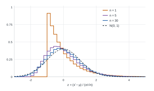
In practice, that’s what lets you say “my F1 is 0.82 plus or minus 0.01”: the uncertainty on a mean shrinks as $1/\sqrt{n}$ , and we know how to quantify it (M9).

6. Why averaging models reduces error

Intuition. If $B$ models make independent mistakes, their errors cancel out when averaged. But if they all err in the same direction, averaging changes nothing.

For $B$ predictions of variance $\sigma^2$ each, pairwise correlated with coefficient $\rho$ :

$$\mathrm{Var}\left(\frac{1}{B}\sum_{b=1}^B \hat f_b\right) = \rho\,\sigma^2 + \frac{1 - \rho}{B}\,\sigma^2$$

The second term vanishes as $B$ grows; the first one stays. That’s the whole idea of random forests (part 17): average many trees (large $B$ ) while making them as different as possible (small $\rho$ ).

It’s also the tool behind part 13’s bias/variance decomposition. Expanding $\mathbb{E}\big[(y - \hat f)^2\big]$ with $y = f + \varepsilon$ , adding and subtracting $\mathbb{E}[\hat f]$ and using the independence of the noise, the cross terms have zero expectation and what’s left is bias² + variance + $\sigma^2$ .

7. Autocorrelation: how a signal resembles a shifted copy of itself

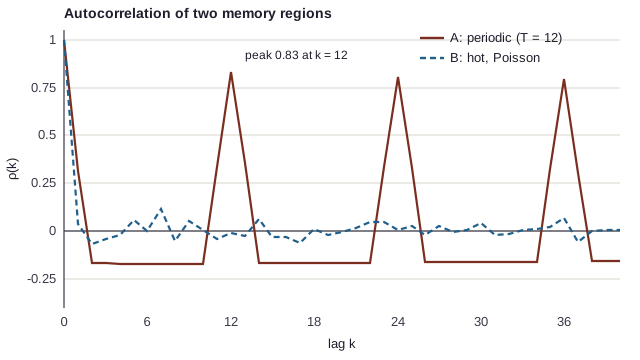
Intuition. To know whether a memory region has a rhythm, compare its access series with the same series shifted by $k$ steps. If it’s periodic with period $T$ , the resemblance is strong for $k = T, 2T, 3T, \dots$

$$\rho(k) = \frac{\sum_t (a_t - \bar a)(a_{t+k} - \bar a)}{\sum_t (a_t - \bar a)^2}$$

It’s the correlation between the series and its shifted version. And it’s exactly the tool that was missing in M1 and M3: Euclidean distance and PCA couldn’t see that a shifted region had the same rhythm; autocorrelation ignores the shift.

---

Code example

Common distributions: theory vs simulation

import numpy as np

rng = np.random.default_rng(0)
N = 200_000

dists = {
    "Bernoulli(p=0.3)": (rng.binomial(1, 0.3, N), 0.3, 0.3 * 0.7),
    "Binomial(n=20, p=0.3)": (rng.binomial(20, 0.3, N), 6.0, 20 * 0.3 * 0.7),
    "Poisson(λ=2)": (rng.poisson(2, N), 2.0, 2.0),
    "Normal(μ=1, σ=2)": (rng.normal(1, 2, N), 1.0, 4.0),
    "Exponential(λ=0.5)": (rng.exponential(2, N), 2.0, 4.0),
}
for name, (sample, mu, var) in dists.items():
    print(f"{name:<24} mean {sample.mean():6.3f} (theory {mu:5.2f}) | variance {sample.var():6.3f} (theory {var:5.2f})")

# Zipf: a few regions get most of the accesses
regions = rng.zipf(1.5, N)
_, counts = np.unique(regions, return_counts=True)
top10_share = np.sort(counts)[::-1][:10].sum() / N
print(f"Zipf(1.5): the 10 most accessed regions get {top10_share:.0%} of the accesses")

With 200,000 draws, every empirical mean and variance lands within 1% of theory (for example 2.004 and 2.007 for Poisson(2), whose expectation and variance are both 2). For Zipf(1.5), the 10 most accessed regions get 76% of the accesses.

Large numbers and the CLT

import numpy as np

rng = np.random.default_rng(0)

# law of large numbers
x = rng.binomial(1, 0.3, 10_000)
running_mean = np.cumsum(x) / np.arange(1, len(x) + 1)
for k in (10, 100, 1000, 10_000):
    print(f"mean of the first {k:>6} draws: {running_mean[k - 1]:.4f}")

# central limit theorem on a very skewed distribution (exponential, mean 2, std 2)
for n in (1, 5, 30, 200):
    means = rng.exponential(2, (50_000, n)).mean(axis=1)
    z = (means - 2) / (2 / np.sqrt(n))
    skew = np.mean(z**3)
    print(f"n={n:<4} std of the means {means.std():.3f} (theory {2 / np.sqrt(n):.3f}) | skewness {skew:5.2f}")

The running mean is 0.4000 after 10 draws, 0.3700 after 100, 0.3220 after 1,000 and 0.3001 after 10,000: it converges to $p = 0.3$ .

$n$	Std of the means	Theory $\sigma/\sqrt n$	Skewness
1	2.012	2.000	2.06
5	0.902	0.894	0.96
30	0.366	0.365	0.36
200	0.141	0.141	0.12

The standard deviation closely follows $\sigma/\sqrt n$ , and the skewness (0 for a Gaussian) melts roughly like $2/\sqrt n$ (0.89, 0.37 and 0.14 in theory): at $n = 30$ , the distribution of the means is already nearly symmetric, while the original distribution isn’t at all.

Averaging correlated models

import numpy as np

rng = np.random.default_rng(0)
sigma2, B = 1.0, 25
for rho in (0.0, 0.3, 0.7):
    cov = sigma2 * (rho * np.ones((B, B)) + (1 - rho) * np.eye(B))
    preds = rng.multivariate_normal(np.zeros(B), cov, 50_000)
    print(f"ρ={rho}: variance of the mean of {B} models = {preds.mean(axis=1).var():.3f} "
          f"(theory {rho * sigma2 + (1 - rho) * sigma2 / B:.3f})")

Correlation $\rho$	Variance of the mean of 25 models	Theory
0	0.040	0.040
0.3	0.327	0.328
0.7	0.703	0.712

With independent models, averaging 25 of them divides the variance by 25. With a correlation of 0.7, you gain almost nothing.

Detecting a period with autocorrelation

import numpy as np

rng = np.random.default_rng(0)


def autocorr(a, max_lag):
    a = a - a.mean()
    var = a @ a
    return np.array([1.0] + [(a[:-k] @ a[k:]) / var for k in range(1, max_lag + 1)])


T = 600
t = np.arange(T)
periodic = ((t % 12) < 2) * rng.poisson(6, T)          # active 2 aggregations out of 12
hot = rng.poisson(3, T).astype(float)
for name, a in (("periodic", periodic), ("hot", hot)):
    ac = autocorr(a.astype(float), 40)
    k_max = 1 + np.argmax(ac[1:])
    print(f"{name:<9}: autocorrelation peak at lag {k_max:>2} (value {ac[k_max]:.2f})")

The periodic region peaks at $k = 12$ with value 0.83 (then 0.80 at $k = 24$ and 0.79 at $k = 36$ ): we recover its period without knowing it. The hot region has no notable peak: its maximum, 0.12 at lag 7, is isolated and doesn’t repeat at multiples of 7 (0.07 at $k = 14$ , 0.02 at $k = 21$ ); it’s noise. The lag of the first autocorrelation peak is a shift-invariant feature: exactly what M1’s and M3’s profiles needed.

---

Hands-on exercise

1. By hand. Compute the expectation and variance of a 6-sided die. Check with a simulation of 100,000 rolls.
2. Variance of a sum. Show that $\mathrm{Var}(X + Y) = \mathrm{Var}(X) + \mathrm{Var}(Y) + 2\,\mathrm{Cov}(X, Y)$ . What does it become if $Y = -X$ ? Check numerically.
3. Zero correlation, yet dependent. Draw $X \sim \mathcal{N}(0, 1)$ and set $Y = X^2$ . Compute their empirical correlation. What do you conclude?
4. How many examples? A region is accessed with an unknown probability $p \approx 0.3$ per aggregation. How many aggregations must you observe for the standard deviation of the estimate $\hat p$ to be below 0.01?
5. Running project. Add to part 14’s features the autocorrelation peak value and its lag, computed on a sliding window of 100 aggregations. Do these two features separate periodic regions from bursts better than periode_estimee?

Hint for question 4: $\mathrm{Var}(\hat p) = p(1-p)/n$ .

---

Further resources

• Blitzstein and Hwang, Introduction to Probability and Harvard’s Stat 110 course, free online: the best introduction to probability.
• Deisenroth et al., Mathematics for Machine Learning, chapter 6 (probability and distributions).
• Seeing Theory (Brown University): interactive visualizations of expectation, variance and the CLT.
• Breslau et al., Web Caching and Zipf-like Distributions (INFOCOM 1999): Zipf applied to caches.

---

What you should be able to do before moving on

• Compute the expectation and variance of a simple discrete distribution
• Match each common distribution to a phenomenon (labels, counts, waiting times, popularity)
• Explain the difference between zero correlation and independence
• State the law of large numbers and the CLT, and explain the $1/\sqrt n$
• Explain with $\rho\sigma^2 + (1-\rho)\sigma^2/B$ why we average decorrelated models
• Compute an autocorrelation and infer a period from it

Next part: M8 · Likelihood, Bayes and entropy. Where MSE and cross-entropy come from: loss functions seen as probabilities.