October 15, 2026 · 17 min read

M9 · Inferential statistics for comparing models

Confidence intervals, bootstrap, McNemar, corrected t and Kolmogorov-Smirnov: proving one model is really better than another, and detecting drift.

Mastering AI · Required Maths · Week 3 (probability and statistics) · Part 9

Goal of this step

“LightGBM gets an F1 of 0.681, logistic regression 0.582: LightGBM is better.” That sentence is worthless until you know whether the gap is bigger than the noise. A test score is an estimate computed on a finite sample: with another test set, it would have been different. This article gives you the tools to claim “A is better than B” with rigor you can defend in front of a thesis jury.

By the end of this article you’ll be able to:

explain what an estimator, its bias and its standard error are;
build a confidence interval and say what “95%” really means;
build an interval by bootstrap for any metric (F1 included);
set up a hypothesis test and interpret a p-value without misreading it;
compare two models on the same test set (paired bootstrap, McNemar) and across several cross-validation folds (corrected t, 5x2cv, Wilcoxon);
detect drift with Kolmogorov-Smirnov and beware of multiple comparisons.

Key concepts

1. Estimator, bias and standard error

Intuition. The F1 you measure on your test set isn’t “the model’s F1”: it’s an estimate of how it would perform on every possible memory region. Change the test set and the number moves. The standard error measures how much it typically moves.

An estimator $\hat\theta$ is a function of the data that targets an unknown quantity $\theta$ . Two properties matter:

the bias $\mathbb{E}[\hat\theta] - \theta$ : is it wrong on average?;
the standard error $\mathrm{SE}(\hat\theta) = \sqrt{\mathrm{Var}(\hat\theta)}$ : how much does it fluctuate from one sample to the next?

For an accuracy measured on $n$ examples, each prediction is either correct or not: it’s a Bernoulli with parameter $p$ (M7). The accuracy is their mean, so:

$\mathrm{SE}(\hat p) = \sqrt{\frac{p(1 - p)}{n}}$

An accuracy of 0.80 measured on 200 examples has a standard error of about 0.028: the second decimal is already uncertain.

2. The confidence interval, and what it really means

Intuition. Instead of a single number, give a range. Thanks to the central limit theorem (M7), a mean approximately follows a normal distribution, and 95% of a normal distribution’s mass lies within $\pm 1.96$ standard deviations of its center:

$\bar x \pm 1.96\,\frac{s}{\sqrt{n}}$

where $s$ is the sample standard deviation. For a proportion, $s/\sqrt n$ becomes $\sqrt{\hat p(1 - \hat p)/n}$ (the Wald interval).

What “95%” means. It is not “there’s a 95% chance the true value is in this interval”. The true value is fixed; the interval is what’s random. The correct statement: if you repeated the experiment many times, 95% of the intervals built this way would contain the true value. We check it by simulation below.

The width shrinks as $1/\sqrt n$ : to divide the uncertainty by 10, you need 100 times more test examples.

3. The bootstrap: intervals without a formula

Intuition. For F1, AUC or a median, there’s no simple standard-error formula. Efron’s idea (1979): the test set is our best picture of the population. Resample with replacement $n$ examples from the $n$ in the test set, recompute the metric, and repeat $B$ times (typically $B = 1{,}000$ to $10{,}000$ ). The spread of the $B$ values mimics the spread you’d have seen with fresh test sets.

The 95% percentile interval is simply:

$\Big[\, q_{2.5\%}\big(\hat\theta^{*}_1, \dots, \hat\theta^{*}_B\big),\ q_{97.5\%}\big(\hat\theta^{*}_1, \dots, \hat\theta^{*}_B\big) \,\Big]$

An important limit: the bootstrap assumes independent examples. Successive aggregations of the same memory region are autocorrelated (M7): you then have to resample by blocks (whole regions, or time slices) rather than example by example.

4. Hypothesis tests and p-values

Intuition. Play devil’s advocate: assume there’s no difference (the null hypothesis $H_0$ ) and ask whether what you observed would be surprising in that world.

The p-value is the probability, if $H_0$ is true, of observing a result at least as extreme as the one you got.
If $p < \alpha$ (often $\alpha = 0.05$ ), you reject $H_0$ .

Two ways to be wrong:

	$H_0$ true (no difference)	$H_0$ false (real difference)
Reject $H_0$	Type I error (false positive), probability $\alpha$	Right call, probability = power $1 - \beta$
Don’t reject	Right call	Type II error (false negative), probability $\beta$

Three misreadings to avoid:

the p-value is not $P(H_0 \mid \text{data})$ . It’s $P(\text{data at least as extreme} \mid H_0)$ : reversing the arrow would take Bayes and a prior (M8);
“not significant” doesn’t mean “no difference”: the test may have lacked power (too few examples);
“significant” doesn’t mean “important”: with a million examples, an F1 gap of 0.001 becomes significant. Always look at the effect size and its interval, not just $p$ .

5. Comparing two models on the same test set

Intuition. Both models are evaluated on the same examples. Easy examples are solved by both, very hard ones missed by both: those examples say nothing about the difference. You must exploit this pairing, or the difference drowns in the shared noise.

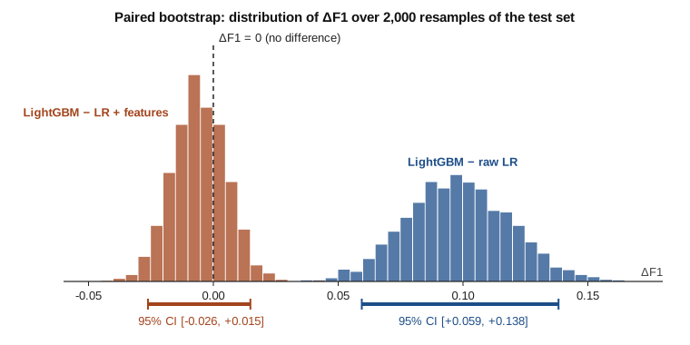
Paired bootstrap. At each resample, draw the same indices for both models and directly compute $\Delta F_1 = F_1^{B} - F_1^{A}$ . If the interval of $\Delta F_1$ excludes 0, the difference is significant.

McNemar’s test. Look only at the disagreements: $n_{01}$ examples where A is right and B wrong, $n_{10}$ where it’s the other way round. Under $H_0$ , each disagreement leans either way with probability $1/2$ , so $n_{01}$ follows a binomial $\mathcal{B}(n_{01} + n_{10}, 1/2)$ . For large counts, use the approximation:

$\chi^2 = \frac{\big(|n_{01} - n_{10}| - 1\big)^2}{n_{01} + n_{10}} \sim \chi^2_1$

It’s the test Dietterich (1998) recommends when each model can only be trained once.

Paired bootstrap: distribution of ΔF1 over 2,000 resamples of the test set. LightGBM − raw LR: distribution entirely to the right of 0, 95% CI +0.059, +0.138. LightGBM − LR + features: distribution centered on 0, 95% CI −0.026, +0.015.

6. Comparing across several cross-validation folds

Intuition. With cross-validation, you get one difference $d_j$ per fold. The reflex is a paired t-test on these differences. Problem: the folds share a large part of their training data, so the $d_j$ are correlated and their variance is underestimated. The naive t-test is far too optimistic (M7 warned us: correlation stops the variance from falling as $1/n$ ).

Two classic corrections, for $J$ differences $d_j$ with mean $\bar d$ and sample variance $\hat\sigma^2$ :

\begin{aligned} t_{\text{naive}} &= \frac{\bar d}{\sqrt{\hat\sigma^2 / J}} \\ t_{\text{corrected}} &= \frac{\bar d}{\sqrt{\left(\frac{1}{J} + \frac{n_{\text{test}}}{n_{\text{train}}}\right)\hat\sigma^2}} \end{aligned}

Nadeau and Bengio’s corrected t (2003) adds the $n_{\text{test}}/n_{\text{train}}$ term to account for the overlap; it’s compared with a Student distribution with $J - 1$ degrees of freedom.

Dietterich’s 5x2cv: 5 repetitions of a 2-fold cross-validation. For repetition $i$ , write $d_i^{(1)}, d_i^{(2)}$ for the two differences, $\bar d_i$ for their mean and $s_i^2 = (d_i^{(1)} - \bar d_i)^2 + (d_i^{(2)} - \bar d_i)^2$ . Then:

$t_{5\times 2} = \frac{d_1^{(1)}}{\sqrt{\frac{1}{5}\sum_{i=1}^{5} s_i^2}}$

approximately follows a Student distribution with 5 degrees of freedom.

Finally, the Wilcoxon (signed-rank) test doesn’t assume a normal distribution: it only looks at the sign and rank of the differences. With 10 differences that are all positive, its exact p-value is $2/2^{10} \approx 0.002$ : the smallest $p$ possible with 10 folds.

7. Kolmogorov-Smirnov to detect drift

Intuition. In production, the distribution of the features can change (new workload, new kernel version). The two-sample Kolmogorov-Smirnov test compares two whole distributions, not just their means. Its statistic is the largest gap between the two empirical cumulative distribution functions:

$D = \max_x \big|F_{\text{ref}}(x) - F_{\text{prod}}(x)\big|$

$D$ measures the size of the drift (between 0 and 1); the p-value only says whether it’s detectable. With lots of data, the slightest drift becomes significant: in monitoring (part 28), you alert on a threshold on $D$ , not on $p < 0.05$ .

8. Multiple comparisons

Intuition. If you run 20 tests at $\alpha = 0.05$ while nothing is true, you get one false positive on average. The probability of getting at least one is:

$1 - (1 - \alpha)^m = 1 - 0.95^{20} \approx 64\%$

That’s the classic tuning trap: try 20 hyperparameter variants on the same test set and keep “the best one”. The Bonferroni correction tests each hypothesis at level $\alpha / m$ : simple, conservative, and it brings the overall risk back under $\alpha$ . Even better: keep a test set you only look at once (part 18).

Code example

Confidence interval of an accuracy, and its coverage

import numpy as np

rng = np.random.default_rng(0)
p_true = 0.80                      # the model's true accuracy (unknown in practice)

# 1. a single test set of 200 examples
correct = rng.binomial(1, p_true, 200)     # 1 = correct prediction
acc = correct.mean()
se = np.sqrt(acc * (1 - acc) / 200)
print(f"accuracy = {acc:.3f} | standard error = {se:.4f} | 95% CI = [{acc - 1.96 * se:.3f}, {acc + 1.96 * se:.3f}]")

# 2. the width of the interval as a function of n
for n in (200, 2_000, 20_000):
    print(f"n = {n:>6}: half-width ≈ ±{1.96 * np.sqrt(p_true * (1 - p_true) / n):.3f}")

# 3. what does "95%" mean? repeat the experiment 10,000 times
n, covered = 200, 0
for _ in range(10_000):
    a = rng.binomial(1, p_true, n).mean()
    s = np.sqrt(a * (1 - a) / n)
    covered += (a - 1.96 * s <= p_true <= a + 1.96 * s)
print(f"coverage rate: {covered / 10_000:.1%}")

Result:

the first test set gives an accuracy of 0.725, a standard error of 0.0316 and the interval $[0.663, 0.787]$ . Bad luck: it doesn’t contain the true value 0.80. That’s exactly what “95%” allows: about one interval in twenty misses the target, and you never know which one;
the half-width is $\pm 0.055$ for 200 examples, $\pm 0.018$ for 2,000 and $\pm 0.006$ for 20,000: $\times 10$ in data, $\div \sqrt{10} \approx 3.2$ in uncertainty;
over 10,000 repetitions, 94.0% of the intervals contain 0.80. Slightly under 95%: the Wald interval is a bit too narrow for a proportion with $n = 200$ (exercise 2 offers something better).

The running project: three models, one test set

We generate synthetic memory regions. A region is hot in the next window if it was accessed a lot recently, if its last access is close, or if it’s periodic and its peak is coming up. That last rule is an interaction: a tree finds it on its own, a logistic regression only sees it if you hand it over.

import numpy as np
import lightgbm as lgb
from scipy import stats
from sklearn.linear_model import LogisticRegression
from sklearn.metrics import f1_score
from sklearn.model_selection import train_test_split


def make_regions(n, rng):
    """Synthetic memory regions: label 1 = hot in the next window."""
    rate = rng.gamma(0.6, 4, n)                          # very uneven popularity
    recent_accesses = rng.poisson(rate)
    since_last = np.round(rng.exponential(30 / (1 + recent_accesses)), 1)
    periodic = rng.binomial(1, 0.25, n)
    before_peak = rng.integers(0, 12, n)                 # steps left before the next peak
    logit = (0.9 * np.log1p(recent_accesses) - 0.05 * since_last
             + 3.0 * periodic * (before_peak < 3) - 1.5 + rng.normal(0, 0.8, n))
    X = np.column_stack([recent_accesses, since_last, periodic, before_peak])
    return X, (logit > 0).astype(int)


def domain_features(X):
    """What a human would add: log of accesses and the "periodic and peak imminent" interaction."""
    return np.column_stack([np.log1p(X[:, 0]), X[:, 1], X[:, 2], X[:, 2] * (X[:, 3] < 3)])


rng = np.random.default_rng(0)
X, y = make_regions(5000, rng)
Xtr, Xte, ytr, yte = train_test_split(X, y, test_size=0.3, random_state=0, stratify=y)

preds = {
    "raw LR": LogisticRegression(max_iter=1000).fit(Xtr, ytr).predict(Xte),
    "LR + features": LogisticRegression(max_iter=1000).fit(domain_features(Xtr), ytr).predict(domain_features(Xte)),
    "LightGBM": lgb.LGBMClassifier(n_estimators=200, learning_rate=0.05, num_leaves=15,
                                   verbose=-1).fit(Xtr, ytr).predict(Xte),
}

# paired bootstrap: resample the SAME indices for every model
B, n_test = 2000, len(yte)
idx = rng.integers(0, n_test, (B, n_test))
f1_boot = {name: np.array([f1_score(yte[i], p[i]) for i in idx]) for name, p in preds.items()}
for name, p in preds.items():
    lo, hi = np.percentile(f1_boot[name], [2.5, 97.5])
    print(f"{name:<14} F1 = {f1_score(yte, p):.3f}  95% bootstrap CI [{lo:.3f}, {hi:.3f}]")


def compare(a, b):
    diff = f1_boot[b] - f1_boot[a]
    lo, hi = np.percentile(diff, [2.5, 97.5])
    ok_a, ok_b = preds[a] == yte, preds[b] == yte
    n01, n10 = int(np.sum(ok_a & ~ok_b)), int(np.sum(~ok_a & ok_b))   # disagreements
    p_mcnemar = stats.binomtest(n01, n01 + n10, 0.5).pvalue
    print(f"{b} − {a}: ΔF1 = {f1_score(yte, preds[b]) - f1_score(yte, preds[a]):+.3f}, "
          f"95% CI [{lo:+.3f}, {hi:+.3f}] | McNemar: {n01} vs {n10}, p = {p_mcnemar:.2g}")


compare("raw LR", "LightGBM")
compare("LR + features", "LightGBM")

About 22% of the regions are hot. On the 1,500 test regions:

Model	F1	95% bootstrap CI
raw LR	0.582	$[0.535, 0.629]$
LR + features	0.686	$[0.645, 0.727]$
LightGBM	0.681	$[0.639, 0.723]$

Comparison	$\Delta F_1$	95% paired CI	McNemar ( $n_{01}$ vs $n_{10}$ )	p
LightGBM − raw LR	+0.099	$[+0.059, +0.138]$	44 vs 84	0.00052
LightGBM − LR + features	−0.005	$[-0.026, +0.015]$	28 vs 25	0.78

Two very different conclusions:

LightGBM clearly beats raw LR: the paired interval is far from 0 and McNemar gives $p = 0.0005$ . Of the 128 regions where the two models disagree, LightGBM is right 84 times;
LightGBM and LR with the right features are tied: the 0.005 gap is lost in the noise ( $p = 0.78$ ). Claiming “LR does better” would be wrong, and so would “LightGBM is useless”: this test set can’t separate them.

Notice the power of pairing too: the individual intervals of the last two models are about 0.08 wide, but the interval of their difference is only 0.04 wide. Comparing two overlapping intervals isn’t a test: only the interval of the difference counts.

Several folds: naive t, corrected t, 5x2cv and Wilcoxon

# continues the previous block (make_regions, X, y already defined)
from sklearn.model_selection import StratifiedKFold

diffs = np.zeros((5, 2))
for r in range(5):
    folds = StratifiedKFold(n_splits=2, shuffle=True, random_state=r).split(X, y)
    for k, (tr, te) in enumerate(folds):
        f_lr = f1_score(y[te], LogisticRegression(max_iter=1000).fit(X[tr], y[tr]).predict(X[te]))
        f_gb = f1_score(y[te], lgb.LGBMClassifier(n_estimators=200, learning_rate=0.05, num_leaves=15,
                                                  verbose=-1).fit(X[tr], y[tr]).predict(X[te]))
        diffs[r, k] = f_gb - f_lr

d = diffs.ravel()
t_naive = d.mean() / (d.std(ddof=1) / np.sqrt(len(d)))
t_nb = d.mean() / np.sqrt((1 / len(d) + 1.0) * d.var(ddof=1))     # Nadeau-Bengio, n_test/n_train = 1
s2 = ((diffs - diffs.mean(axis=1, keepdims=True)) ** 2).sum(axis=1)
t_5x2 = diffs[0, 0] / np.sqrt(s2.mean())                            # Dietterich, 5 dof
print(f"mean ΔF1 over 10 folds = {d.mean():+.3f} (min {d.min():+.3f}, max {d.max():+.3f})")
print(f"naive t     = {t_naive:5.2f}, p = {2 * stats.t.sf(abs(t_naive), 9):.2g}")
print(f"corrected t = {t_nb:5.2f}, p = {2 * stats.t.sf(abs(t_nb), 9):.2g}")
print(f"5x2cv t     = {t_5x2:5.2f}, p = {2 * stats.t.sf(abs(t_5x2), 5):.2g}")
print(f"Wilcoxon    : p = {stats.wilcoxon(d).pvalue:.2g}")

Over the 10 folds, LightGBM beats raw LR by $+0.083$ on average (between $+0.054$ and $+0.095$ depending on the fold).

Test	Statistic	p
Naive paired t (9 dof)	20.82	$6.4 \times 10^{-9}$
Nadeau-Bengio corrected t (9 dof)	6.28	0.00014
Dietterich 5x2cv t (5 dof)	6.07	0.0018
Wilcoxon signed-rank	—	0.002

All four tests agree on the direction, but the naive t is three times too confident (20.8 versus 6.3): it treats 10 overlapping folds as 10 independent experiments. Here the effect is big enough that the decision doesn’t change. On a finer gap, the naive t would call significant something that isn’t: that’s why you use the corrected t or 5x2cv in a thesis.

Drift and multiple comparisons

import numpy as np
from scipy import stats

rng = np.random.default_rng(0)

# drift: time since last access, before and after a workload change
reference = rng.exponential(10, 2000)          # training week
same_dist = rng.exponential(10, 2000)          # following week, nothing changed
drifted = rng.exponential(12, 2000)            # new workload: accesses 20% further apart
for name, x in (("same", same_dist), ("drifted", drifted)):
    res = stats.ks_2samp(reference, x)
    print(f"{name:<8}: D = {res.statistic:.3f}, p = {res.pvalue:.2g}")

# multiple comparisons: 20 pure-noise features tested against the label
n_exp, m, alpha = 2000, 20, 0.05
at_least_one, at_least_one_bonf = 0, 0
for _ in range(n_exp):
    label = rng.binomial(1, 0.3, 200)
    noise = rng.normal(size=(200, m))
    p = np.array([stats.ttest_ind(noise[label == 1, j], noise[label == 0, j]).pvalue for j in range(m)])
    at_least_one += (p < alpha).any()
    at_least_one_bonf += (p < alpha / m).any()
print(f"at least one false positive: {at_least_one / n_exp:.1%} (theory {1 - (1 - alpha) ** m:.1%}) | "
      f"with Bonferroni: {at_least_one_bonf / n_exp:.1%}")

Same distribution: $D = 0.022$ , $p = 0.74$ , nothing to report. Drift of 20% on the mean: $D = 0.072$ , $p = 6.2 \times 10^{-5}$ , detected with 2,000 points per week.
Multiple comparisons: with 20 pure-noise features, 64.0% of experiments find at least one “significant” feature (theory says 64.2%). With Bonferroni ( $\alpha / 20 = 0.0025$ ), it drops back to 5.5%.

Hands-on exercise

By hand. A model has an accuracy of 0.80. How many test examples do you need for the half-width of the 95% confidence interval to be under 0.01? And under 0.001?
A better interval. Redo the coverage simulation with $n = 30$ and a true accuracy of 0.95. Compare the coverage of the Wald interval with that of the Wilson interval (stats.binomtest(k, n).proportion_ci(method="wilson")). Which one keeps its promise?
Bootstrap other metrics. On the running project’s test set, build bootstrap intervals for LightGBM’s precision and recall. Which is wider, and why? (Hint: how many examples is each one computed on?)
Little data. Redo the 5x2cv with make_regions(600, ...) instead of 5,000, for LightGBM against raw LR then against LR + features. Do the conclusions hold? What do the naive t and the corrected t say?
Running project. On part 14’s dataset, split the trace into two time halves and apply Kolmogorov-Smirnov to each feature. How many features drift at the 0.05 level, then after Bonferroni? Rank them by $D$ rather than by $p$ .

Hint for question 1: $n = 1.96^2 \times 0.8 \times 0.2 / 0.01^2$ , i.e. about 6,150 examples. For 0.001, a hundred times more.

Further resources

Dietterich, Approximate Statistical Tests for Comparing Supervised Classification Learning Algorithms (Neural Computation, 1998): McNemar and 5x2cv.
Nadeau and Bengio, Inference for the Generalization Error (Machine Learning, 2003): the corrected t.
Efron and Tibshirani, An Introduction to the Bootstrap (1993).
Demšar, Statistical Comparisons of Classifiers over Multiple Data Sets (JMLR, 2006): Wilcoxon, Friedman and multiple comparisons.
Wasserstein and Lazar, The ASA Statement on p-Values (2016): what a p-value says, and what it doesn’t.

What you should be able to do before moving on

Compute the standard error of an accuracy and explain the $1/\sqrt n$ decay
Build a confidence interval and state correctly what “95%” means
Build a bootstrap interval for a metric with no formula (F1, AUC)
Define p-value, type I error, type II error and power
Compare two models on the same test set with a paired bootstrap and McNemar
Explain why the naive t-test on folds is too optimistic, and use the corrected t or 5x2cv
Detect drift with Kolmogorov-Smirnov and correct for multiple comparisons

Next part: M10 · Gradient descent and its variants. How you actually find the minimum of all these loss functions.