M8 · Likelihood, Bayes and entropy

Mastering AI · Required Maths · Week 3 (probability and statistics) · Part 8

Goal of this step

So far we’ve taken MSE and log-loss as given. They don’t fall from the sky: they follow from a single idea, maximum likelihood. Add Bayes’ theorem and the notion of entropy, and you also get $L_2$ regularization and the splitting criterion of decision trees.

By the end of this article you’ll be able to:

• apply Bayes’ theorem and explain the effect of the prior;
• estimate a parameter by maximum likelihood;
• derive MSE from Gaussian noise and cross-entropy from a Bernoulli label;
• interpret $L_2$ regularization as a Gaussian prior (MAP);
• compute entropy, cross-entropy, KL divergence and information gain.

---

Key concepts

1. Bayes’ theorem

Intuition. We often know $P(\text{clue} \mid \text{cause})$ (“if the region is cold, my detector says so 95% of the time”) but we want $P(\text{cause} \mid \text{clue})$ (“the detector says cold: what’s the chance it really is?”). Bayes reverses the arrow, provided you know the base rate, the prior.

$$\begin{aligned} P(A \mid B) &= \frac{P(B \mid A)\,P(A)}{P(B)} \\ P(B) &= P(B \mid A)P(A) + P(B \mid \bar A)P(\bar A) \end{aligned}$$

Running-project example: 70% of regions are cold. A detector says “cold” for 95% of cold regions and, by mistake, for 20% of hot ones. When it says “cold”, the probability that the region is actually hot (a false cold) is:

$$\begin{aligned} P(\text{hot} \mid \text{says cold}) &= \frac{0.20 \times 0.30}{0.95 \times 0.70 + 0.20 \times 0.30} \\ &= \frac{0.06}{0.725} \approx 8.3\,\% \end{aligned}$$

The same detector, on a workload where only 20% of regions are cold, gives 46% false colds. A classifier’s quality can never be read without the base rate: we’ll see it again in part 15 with precision.

2. Likelihood

Intuition. You have data and a model with a parameter $\theta$ . The likelihood $L(\theta)$ is the probability of having observed exactly this data if the parameter were $\theta$ . Maximum likelihood (MLE) picks the $\theta$ that makes the data most probable.

For independent observations, the likelihood is a product, which the logarithm turns into a sum (numerically more stable, same maximum):

$$\hat\theta = \arg\max_\theta \sum_{i=1}^n \log p(x_i \mid \theta)$$

Example: access counts assumed to follow a Poisson( $\lambda$ ) distribution. Setting the derivative of the log-likelihood to zero gives $\hat\lambda = \bar x$ : the maximum likelihood estimator is the sample mean.

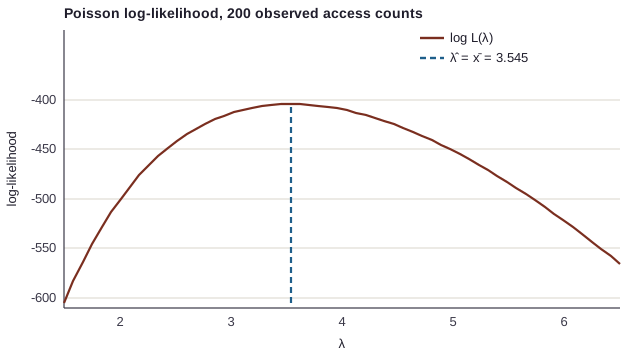
Minimizing a loss means maximizing a likelihood. In ML we write everything as a minimization: the loss is the average negative log-likelihood (NLL).

3. Gaussian noise ⇒ MSE

Assumption: $y_i = w^\top x_i + \varepsilon_i$ with independent noise $\varepsilon_i \sim \mathcal{N}(0, \sigma^2)$ . The NLL is:

$$-\log L(w, \sigma) = \frac{n}{2}\log(2\pi\sigma^2) + \frac{1}{2\sigma^2}\sum_{i=1}^n \big(y_i - w^\top x_i\big)^2$$

For fixed $\sigma$ , only the second term depends on $w$ : it’s the sum of squared errors. Maximizing the Gaussian likelihood is exactly minimizing the MSE. And the estimator of $\sigma$ is the square root of the MSE.

Corollary: MSE assumes symmetric noise without extreme values. With outliers, a Laplace distribution gives the loss $|y - \hat y|$ (MAE), which is more robust.

4. Bernoulli label ⇒ cross-entropy

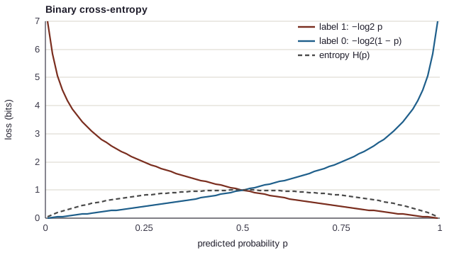
Assumption: $y_i \in \{0, 1\}$ follows a Bernoulli distribution with parameter $p_i = \sigma(w^\top x_i)$ . The probability of a label is $p_i^{y_i}(1 - p_i)^{1 - y_i}$ , hence:

$$-\log L(w) = -\sum_{i=1}^n \big[y_i \log p_i + (1 - y_i)\log(1 - p_i)\big]$$

That’s exactly the log-loss (or binary cross-entropy) of logistic regression. It punishes a confident wrong prediction very hard: predicting $p = 0.01$ for a region that will be accessed costs $-\log_2 0.01 \approx 6.6$ bits.

5. MAP: regularization as a prior

Intuition. Before seeing the data, you may already have an opinion: “the weights are probably small”. Bayes lets you combine that prior with the likelihood. You then maximize the posterior probability (MAP):

$$\hat w_{\text{MAP}} = \arg\max_w \big[\log p(\text{data} \mid w) + \log p(w)\big]$$

With a Gaussian prior $w \sim \mathcal{N}(0, \tau^2 I)$ , $\log p(w) = -\frac{\|w\|^2}{2\tau^2} + \text{const}$ : you recover $L_2$ regularization (Ridge), with $\lambda = \sigma^2/\tau^2$ . A Laplace prior would give $L_1$ (Lasso). Regularization isn’t a trick: it’s a prior belief about the weights (M11, part 16).

6. Entropy, cross-entropy and KL divergence

Intuition. Entropy measures the uncertainty of a distribution, in bits: the average number of yes/no questions needed to guess the outcome. A fair coin is worth 1 bit, a rigged coin that always lands heads is worth 0.

$$H(p) = -\sum_k p_k \log_2 p_k$$

Cross-entropy $H(p, q) = -\sum_k p_k \log_2 q_k$ measures the average cost when the truth follows $p$ but you encode (or predict) with $q$ . The gap is the Kullback-Leibler divergence:

$$\begin{aligned} H(p, q) &= H(p) + \mathrm{KL}(p \,\|\, q) \\ \mathrm{KL}(p \,\|\, q) &= \sum_k p_k \log_2 \frac{p_k}{q_k} \geq 0 \end{aligned}$$

KL is zero if and only if $q = p$ , and it isn’t symmetric. Since $H(p)$ doesn’t depend on the model, minimizing cross-entropy is the same as minimizing the KL between the true label distribution and the one the model predicts.

7. The information gain of trees

A decision tree (part 17) picks, at each node, the split that reduces the entropy of the labels the most:

$$\text{gain} = H(\text{node}) - \sum_{\text{children}} \frac{n_{\text{child}}}{n_{\text{node}}}\, H(\text{child})$$

A split that cleanly separates hot regions from cold ones produces “pure” children, with low entropy, hence a high gain.

---

Code example

Bayes and the weight of the prior

p_cold = 0.70               # prior: 70% of regions are cold (Zipf)
p_says_cold_if_cold = 0.95
p_says_cold_if_hot = 0.20
p_says_cold = p_says_cold_if_cold * p_cold + p_says_cold_if_hot * (1 - p_cold)
p_hot_if_says_cold = p_says_cold_if_hot * (1 - p_cold) / p_says_cold
print(f"P(says cold) = {p_says_cold:.3f} | P(actually hot | says cold) = {p_hot_if_says_cold:.3f}")
for prior in (0.9, 0.5, 0.2):
    psc = p_says_cold_if_cold * prior + p_says_cold_if_hot * (1 - prior)
    print(f"  prior cold = {prior:.1f} -> P(hot | says cold) = {p_says_cold_if_hot * (1 - prior) / psc:.3f}")

Share of cold regions	$P(\text{hot} \mid \text{says cold})$
90%	2.3%
70%	8.3%
50%	17.4%
20%	45.7%

Same detector, same error rates: the share of false colds among regions declared cold goes from 2% to 46% depending on the workload.

Maximum likelihood: Poisson, Gaussian and Ridge

import numpy as np
from scipy.optimize import minimize, minimize_scalar
from scipy.special import gammaln

rng = np.random.default_rng(0)

# 1. Poisson: the MLE of λ is the mean
accesses = rng.poisson(3.2, 200)
nll_poisson = lambda lam: -np.sum(accesses * np.log(lam) - lam - gammaln(accesses + 1))
res = minimize_scalar(nll_poisson, bounds=(0.1, 10), method="bounded")
print(f"Poisson: numerical MLE of λ = {res.x:.4f} | sample mean = {accesses.mean():.4f}")

# 2. Gaussian noise => MSE
n, d = 300, 3
X = rng.normal(size=(n, d))
y = X @ np.array([2.0, -1.0, 0.5]) + rng.normal(0, 0.5, n)

def nll_gauss(params):
    w, log_sigma = params[:d], params[d]
    sigma2 = np.exp(2 * log_sigma)
    r = y - X @ w
    return 0.5 * n * np.log(2 * np.pi * sigma2) + (r @ r) / (2 * sigma2)

opt = minimize(nll_gauss, np.zeros(d + 1))
w_ls = np.linalg.lstsq(X, y, rcond=None)[0]
print(f"Gaussian MLE w : {opt.x[:d].round(4)} | MLE σ = {np.exp(opt.x[d]):.4f}")
print(f"least squares w: {w_ls.round(4)} | √(MSE) = {np.sqrt(np.mean((y - X @ w_ls) ** 2)):.4f}")

# 3. MAP with a Gaussian prior => Ridge
lam = 10.0
w_ridge = np.linalg.solve(X.T @ X + lam * np.eye(d), X.T @ y)
w_map = minimize(lambda w: np.sum((y - X @ w) ** 2) + lam * w @ w, np.zeros(d)).x
print(f"Ridge (closed form): {w_ridge.round(4)} | numerical MAP: {w_map.round(4)}")

Method	Result
Poisson MLE (numerical optimization)	$\hat\lambda = 3.5450$
Sample mean	$3.5450$
Gaussian MLE	$w = (2.0067,\ -0.9955,\ 0.4344)$ , $\hat\sigma = 0.5097$
Least squares	$w = (2.0067,\ -0.9955,\ 0.4344)$ , $\sqrt{\text{MSE}} = 0.5097$
Ridge, closed form ( $\lambda = 10$ )	$w = (1.948,\ -0.9622,\ 0.4151)$
Numerical MAP, Gaussian prior	$w = (1.948,\ -0.9622,\ 0.4151)$

Three pairs of methods, three exact matches: the Poisson MLE is the mean, the Gaussian MLE is the least squares solution, and the Gaussian MAP is Ridge regression. Notice too that Ridge shrinks every weight toward 0, as the prior predicts.

Entropy, KL and information gain

import numpy as np


def H(p):
    p = np.asarray(p, float)
    p = p[p > 0]
    return -np.sum(p * np.log2(p))


def CE(p, q):
    return -np.sum(np.asarray(p) * np.log2(q))


def KL(p, q):
    return CE(p, q) - H(p)


p = np.array([0.7, 0.2, 0.1])
q = np.array([0.2, 0.3, 0.5])
print(f"H(p) = {H(p):.3f} bits | H(uniform over 3) = {H([1/3] * 3):.3f} bits")
print(f"CE(p, q) = {CE(p, q):.3f} = H(p) + KL(p||q) = {H(p):.3f} + {KL(p, q):.3f}")
print(f"KL(p||q) = {KL(p, q):.3f} | KL(q||p) = {KL(q, p):.3f}")

# information gain of a split on 100 regions (30 hot, 70 cold)
y_node = np.array([1] * 30 + [0] * 70)
left = np.array([1] * 27 + [0] * 8)                     # depuis_dernier < threshold
right = np.array([1] * 3 + [0] * 62)
Hb = lambda v: H([v.mean(), 1 - v.mean()])
gain = Hb(y_node) - (len(left) * Hb(left) + len(right) * Hb(right)) / len(y_node)
print(f"node entropy {Hb(y_node):.3f} | left {Hb(left):.3f} | right {Hb(right):.3f} | gain {gain:.3f} bits")

• $H(p) = 1.157$ bits, versus $1.585$ for the uniform distribution over 3 values (the maximum possible): $p$ is fairly predictable.
• $H(p, q) = 2.073 = 1.157 + 0.916$ : cross-entropy is indeed entropy plus KL.
• $\mathrm{KL}(p \| q) = 0.916$ but $\mathrm{KL}(q \| p) = 0.975$ : KL isn’t a symmetric distance.
• The split takes the entropy from $0.881$ bits (node) to $0.776$ (left) and $0.270$ (right): a gain of $0.434$ bits. The right branch (62 cold, 3 hot) is almost pure.

---

Hands-on exercise

1. Bayes by hand. A detection test has 99% sensitivity and 99% specificity. If the condition affects 1 person in 1,000, what’s the probability of being affected when the test is positive? Check by simulation.
2. Bernoulli MLE. For $n$ observations in 0/1, write the log-likelihood of $p$ and show that $\hat p$ is the proportion of 1s. Check with minimize_scalar.
3. Laplace and MAE. Show that if the noise follows a Laplace distribution, the NLL is proportional to $\sum |y_i - w^\top x_i|$ . Add 5 outliers to y and compare the weights obtained with MSE and with MAE (scipy.optimize.minimize).
4. KL isn’t symmetric. Find two distributions $p$ and $q$ over 2 values for which $\mathrm{KL}(p\|q)$ and $\mathrm{KL}(q\|p)$ differ by a factor of at least 3.
5. Running project. On part 14’s dataset, compute the information gain of the split depuis_dernier < s for several thresholds $s$ . Which threshold maximizes the gain? Compare with the first split of a DecisionTreeClassifier(criterion="entropy", max_depth=1).

Hint for question 1: the answer is around 9%, not 99%.

---

Further resources

• Bishop, Pattern Recognition and Machine Learning, chapters 1 and 2: likelihood, MAP and Bayes applied to ML.
• Murphy, Probabilistic Machine Learning: An Introduction, chapters 4 and 6 (estimation and information theory), free online.
• 3Blue1Brown, Bayes theorem, the geometry of changing beliefs (video).
• Christopher Olah, Visual Information Theory (colah.github.io blog).

---

What you should be able to do before moving on

• Apply Bayes and explain the effect of the base rate
• Write a log-likelihood and find its maximum
• Derive MSE from Gaussian noise and the log-loss from a Bernoulli label
• Explain $L_2$ regularization as a Gaussian prior
• Compute entropy, cross-entropy and KL, and relate the three
• Compute the information gain of a split

Next part: M9 · Inferential statistics for comparing models. How to claim, with numbers and confidence intervals, that one model is better than another.