M5 · The chain rule and backpropagation

Mastering AI · Required Maths · Week 2 (calculus) · Part 5

Goal of this step

A neural network is a composition of functions: one layer, then another, then another. Training it requires the gradient of the loss with respect to every weight, including those of the first layer, buried under all the others. The chain rule, applied cleverly, gives all of them at once: that’s backpropagation.

By the end of this article you’ll be able to:

• apply the chain rule in one and several variables;
• read a computation graph and push gradients through it by hand;
• write a mini autograd engine in 80 lines and compare it with PyTorch;
• backpropagate by hand through a two-layer MLP;
• explain why gradients vanish in deep sigmoid networks.

---

Key concepts

1. The chain rule

Intuition. If $y$ depends on $u$ and $u$ depends on $x$ , a small change in $x$ propagates: it changes $u$ , which changes $y$ . The rates of change multiply. If $u$ moves 3 times faster than $x$ , and $y$ 2 times faster than $u$ , then $y$ moves 6 times faster than $x$ .

$$\frac{dy}{dx} = \frac{dy}{du} \cdot \frac{du}{dx}$$

Example: $h(x) = \sin(x^2)$ . With $u = x^2$ , $h'(x) = \cos(x^2) \cdot 2x$ . At $x = 1.3$ that’s $-0.309196$ , exactly what M4’s finite difference gives.

2. Several variables: paths add up

Intuition. If $x$ influences $y$ through several paths, the contributions of each path add up.

$$\frac{\partial y}{\partial x} = \sum_{k} \frac{\partial y}{\partial u_k} \cdot \frac{\partial u_k}{\partial x}$$

In matrix form, the partial derivatives of $f : \mathbb{R}^n \to \mathbb{R}^m$ go into the Jacobian matrix $J_{ij} = \partial f_i / \partial x_j$ , of size $m \times n$ . The chain rule becomes a product of Jacobians:

$$J_{f \circ g}(x) = J_f\big(g(x)\big) \cdot J_g(x)$$

That’s M2’s “matrix product = composition”, now applied to the “local” transformations that derivatives are. For a linear layer $z = Wa + b$ , the Jacobian of $z$ with respect to $a$ is simply $W$ .

3. The computation graph

Intuition. Break the loss computation into elementary operations (additions, products, sigmoids, logs). Each operation knows its own local derivative. The final loss is obtained by moving forward through the graph (forward pass); the gradients are obtained by moving backward (backward pass), multiplying the local derivatives.

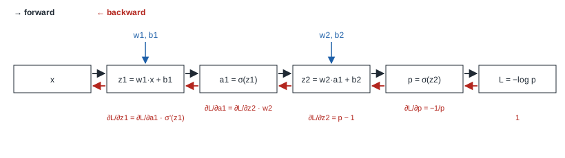
On this small network (one hidden neuron, one output neuron, label $y = 1$ ), the backward pass starts from $\partial L / \partial L = 1$ and climbs back:

• $\partial L / \partial p = -1/p$ ;
• through the sigmoid, $\partial L / \partial z_2 = -\frac{1}{p} \cdot p(1-p) = p - 1$ (the same simplification as in M4);
• through the linear layer, $\partial L / \partial a_1 = (p - 1)\,w_2$ and $\partial L / \partial w_2 = (p - 1)\,a_1$ ;
• and so on down to $w_1$ and $b_1$ .

4. Why “backward”?

Intuition. A loss is a single number, but there are millions of parameters. Starting from the loss and going back, each node is visited once, and at the end you have the gradient with respect to every parameter. The total cost is on the order of the forward pass.

That’s reverse mode automatic differentiation. Forward mode (starting from the inputs) would give the derivative with respect to a single input per pass: one pass per parameter. For a network with a million weights, that’s the difference between 2 passes and a million.

5. Vanishing gradients

Intuition. In an $L$ -layer network, the first layer’s gradient is a product of $L$ factors. If each factor is smaller than 1, the product collapses exponentially.

The sigmoid’s derivative is at most $\sigma'(0) = 1/4$ . Each sigmoid layer therefore multiplies the gradient by a factor often well below 1:

$$\frac{\partial L}{\partial a_1} = \frac{\partial L}{\partial a_L} \prod_{\ell=2}^{L} W_\ell^\top \operatorname{diag}\big(\sigma'(z_\ell)\big)$$

The first layers barely learn anything. It’s the same mechanism as M3’s matrix powers: factors below 1, repeated, wipe out the signal. Two classic fixes, covered in part 22:

• replace the sigmoid with ReLU, whose derivative is 1 on its active part;
• initialize weights at the right scale (He init for ReLU, Xavier for tanh).

---

Code example

A mini-autograd in Python

Each Value remembers its parents and knows how to push its gradient back. backward() sorts the graph and applies the chain rule node by node, from last to first.

import math
import torch


class Value:
    """A number that remembers how it was computed."""

    def __init__(self, data, parents=(), op=""):
        self.data, self.grad = data, 0.0
        self._parents, self._op = parents, op
        self._backward = lambda: None

    def __add__(self, other):
        other = other if isinstance(other, Value) else Value(other)
        out = Value(self.data + other.data, (self, other), "+")
        def _backward():
            self.grad += out.grad            # d(a+b)/da = 1
            other.grad += out.grad           # d(a+b)/db = 1
        out._backward = _backward
        return out

    def __mul__(self, other):
        other = other if isinstance(other, Value) else Value(other)
        out = Value(self.data * other.data, (self, other), "*")
        def _backward():
            self.grad += other.data * out.grad   # d(ab)/da = b
            other.grad += self.data * out.grad   # d(ab)/db = a
        out._backward = _backward
        return out

    def sigmoid(self):
        s = 1 / (1 + math.exp(-self.data))
        out = Value(s, (self,), "σ")
        def _backward():
            self.grad += s * (1 - s) * out.grad
        out._backward = _backward
        return out

    def log(self):
        out = Value(math.log(self.data), (self,), "log")
        def _backward():
            self.grad += (1 / self.data) * out.grad
        out._backward = _backward
        return out

    def backward(self):
        # topological sort: process each node after everything that depends on it
        order, seen = [], set()
        def visit(v):
            if v not in seen:
                seen.add(v)
                for p in v._parents:
                    visit(p)
                order.append(v)
        visit(self)
        self.grad = 1.0
        for v in reversed(order):
            v._backward()


# the network from the figure, with y = 1
x, w1, b1, w2, b2 = Value(0.5), Value(-1.2), Value(0.3), Value(2.0), Value(-0.5)
a1 = (w1 * x + b1).sigmoid()
p = (w2 * a1 + b2).sigmoid()
L = p.log() * -1.0
L.backward()
print(f"mini-autograd: L = {L.data:.5f} | dL/dw1 = {w1.grad:.5f} | dL/db1 = {b1.grad:.5f} | dL/dw2 = {w2.grad:.5f} | dL/db2 = {b2.grad:.5f}")

# the same with PyTorch
t = {k: torch.tensor(v, requires_grad=True, dtype=torch.float64)
     for k, v in dict(w1=-1.2, b1=0.3, w2=2.0, b2=-0.5).items()}
a1t = torch.sigmoid(t["w1"] * 0.5 + t["b1"])
pt = torch.sigmoid(t["w2"] * a1t + t["b2"])
Lt = -torch.log(pt)
Lt.backward()
print("PyTorch      : L = {:.5f} | dL/dw1 = {:.5f} | dL/db1 = {:.5f} | dL/dw2 = {:.5f} | dL/db2 = {:.5f}".format(
    Lt.item(), t["w1"].grad.item(), t["b1"].grad.item(), t["w2"].grad.item(), t["b2"].grad.item()))

	$L$	$\partial L/\partial w_1$	$\partial L/\partial b_1$	$\partial L/\partial w_2$	$\partial L/\partial b_2$
mini-autograd	0.53292	−0.10099	−0.20198	−0.17580	−0.41311
PyTorch	0.53292	−0.10099	−0.20198	−0.17580	−0.41311

Identical to the last digit. Note that $\partial L/\partial w_1 = x \cdot \partial L/\partial b_1 = 0.5 \times (-0.20198)$ : that’s the chain rule through $z_1 = w_1 x + b_1$ .

Backpropagation by hand in an MLP

An MLP with 9 inputs (like our features), 16 sigmoid hidden neurons and one output, on 64 examples. We write the backward pass layer by layer, following the graph.

import numpy as np
import torch

rng = np.random.default_rng(0)
n, d, hdim = 64, 9, 16
X = rng.normal(size=(n, d))
y = (X[:, 0] - X[:, 1] + 0.5 * rng.normal(size=n) > 0).astype(float).reshape(-1, 1)
W1, B1 = rng.normal(0, 0.5, (d, hdim)), np.zeros((1, hdim))
W2, B2 = rng.normal(0, 0.5, (hdim, 1)), np.zeros((1, 1))
sig = lambda z: 1 / (1 + np.exp(-z))

# forward pass
Z1 = X @ W1 + B1
A1 = sig(Z1)
Z2 = A1 @ W2 + B2
P = sig(Z2)
loss = -np.mean(y * np.log(P) + (1 - y) * np.log(1 - P))

# backward pass: climb back up the chain, one layer at a time
dZ2 = (P - y) / n                     # dL/dZ2 (sigmoid + log-loss simplify)
dW2 = A1.T @ dZ2
dB2 = dZ2.sum(axis=0, keepdims=True)
dA1 = dZ2 @ W2.T                      # through layer 2: Jacobian = W2
dZ1 = dA1 * A1 * (1 - A1)             # through the sigmoid
dW1 = X.T @ dZ1
dB1 = dZ1.sum(axis=0, keepdims=True)

# same computation with autograd
T = lambda a: torch.tensor(a, requires_grad=True)
W1t, B1t, W2t, B2t = T(W1), T(B1), T(W2), T(B2)
Pt = torch.sigmoid(torch.sigmoid(torch.tensor(X) @ W1t + B1t) @ W2t + B2t)
losst = torch.nn.functional.binary_cross_entropy(Pt, torch.tensor(y))
losst.backward()
for name, a, b in (("W1", dW1, W1t), ("B1", dB1, B1t), ("W2", dW2, W2t), ("B2", dB2, B2t)):
    print(f"{name}: max hand/autograd gap = {np.abs(a - b.grad.numpy()).max():.1e}")
print(f"loss: hand {loss:.6f} | torch {losst.item():.6f}")

The gaps are around $10^{-16}$ : machine precision. Six lines are enough for an MLP’s backward pass. The pattern repeats for every layer: weight gradient = transposed input activation × output gradient; gradient to pass back = output gradient × transposed weights; through the activation = element-wise multiplication by its derivative.

Vanishing gradients, measured

We stack 20 layers of 32 neurons and measure each layer’s gradient norm after a single backward pass.

import math
import torch


def gradient_norms(activation, depth=20, width=32, seed=0):
    torch.manual_seed(seed)
    layers = []
    for _ in range(depth):
        lin = torch.nn.Linear(width, width)
        gain = 2.0 if activation is torch.nn.ReLU else 1.0   # He init for ReLU (part 22)
        torch.nn.init.normal_(lin.weight, 0, math.sqrt(gain / width))
        torch.nn.init.zeros_(lin.bias)
        layers += [lin, activation()]
    net = torch.nn.Sequential(*layers, torch.nn.Linear(width, 1))
    xb = torch.randn(256, width)
    net(xb).pow(2).mean().backward()
    return [net[2 * i].weight.grad.norm().item() for i in range(depth)]


for act in (torch.nn.Sigmoid, torch.nn.ReLU):
    g = gradient_norms(act)
    print(f"{act.__name__:<8} layer 1: {g[0]:.2e} | layer 10: {g[9]:.2e} | layer 20: {g[19]:.2e}")

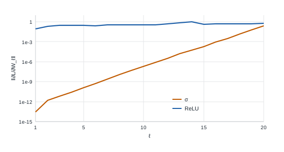
Activation	Layer 1 (input)	Layer 10	Layer 20 (output)
sigmoid	$3.0 \times 10^{-14}$	$2.0 \times 10^{-7}$	$2.4 \times 10^{-1}$
ReLU + He init	$8.7 \times 10^{-2}$	$3.8 \times 10^{-1}$	$6.5 \times 10^{-1}$

With sigmoids, the gradient loses about a factor of 5 per layer: thirteen orders of magnitude between output and input. The first layers will never move. With ReLU and the right initialization, it stays on the same order everywhere.

---

Hands-on exercise

1. By hand. Compute $\frac{d}{dx}\, e^{-x^2/2}$ and $\frac{d}{dx}\,\log\big(1 + e^{3x}\big)$ with the chain rule, then check with a centered difference.
2. Extend the mini-autograd. Add __pow__, tanh and relu to Value, then recompute the small network’s gradients with tanh instead of the sigmoid. Compare with PyTorch.
3. A double path. With your autograd, compute the gradient of $f = a \cdot b + a$ with respect to $a$ . Why do the _backward functions need += rather than =? What happens with =?
4. MLP by hand, with ReLU. Redo the NumPy backpropagation with a ReLU hidden layer instead of the sigmoid. Which line changes? Check with PyTorch.
5. Vanishing gradients. In gradient_norms, use ReLU without He init (gain = 1). What happens to the norms? Also try torch.nn.Tanh.

Hint for question 3: when a value is used twice, the contributions of both paths must add up (section 2).

---

Further resources

• Andrej Karpathy, The spelled-out intro to neural networks and backpropagation: building micrograd (YouTube): the direct inspiration for this article’s mini-autograd.
• 3Blue1Brown, Neural Networks, episodes 3 and 4: backpropagation, animated.
• Christopher Olah, Calculus on Computational Graphs: Backpropagation (colah.github.io).
• Goodfellow, Bengio, Courville, Deep Learning, section 6.5.

---

What you should be able to do before moving on

• Apply the chain rule to a composition of functions
• Explain why the contributions of several paths add up
• Draw a small network’s computation graph and propagate gradients through it by hand
• Write the backward pass of a two-layer MLP in NumPy
• Explain why we backpropagate in reverse mode rather than forward mode
• Explain vanishing gradients and name two fixes

Next part: M6 · Hessian, convexity and Taylor expansion. The gradient gives the slope; the curvature tells whether the slope can be trusted, and why some losses are easy to optimize and others aren’t.