M1 · Vectors, dot product and norms

Mastering AI · Required Maths · Week 1 (linear algebra) · Part 1

Goal of this step

In ML, everything is a vector: an example, a row of features, a model’s weights, an embedding, a gradient. Three operations keep coming back: adding, measuring a length (the norm) and comparing two directions (the dot product).

By the end of this article you’ll be able to:

• read a vector both as a point and as an arrow;
• interpret a dot product as a projection and a measure of alignment;
• choose between the $L_1$ , $L_2$ and $L_\infty$ norms, and between Euclidean distance and cosine similarity;
• spot these objects in linear regression, kNN, regularization and attention.

This is a refresher: we go fast on definitions and insist on geometric intuition, which you’ll use everywhere afterwards.

---

Key concepts

1. A vector: a point and an arrow

Intuition. A list of $n$ numbers, seen two ways: a point in an $n$ -dimensional space, or an arrow from the origin (a direction and a length).

$$x = (x_1, x_2, \dots, x_n) \in \mathbb{R}^n$$

• A row of your dataset is a point in $\mathbb{R}^n$ , with $n$ the number of features. The 9 features from part 14 turn each (region, time) pair into a point in $\mathbb{R}^9$ .
• The weights $w$ of a linear model are an arrow in that same space.

Two basic operations, both component-wise:

• addition: $u + v = (u_1 + v_1, \dots, u_n + v_n)$ , putting arrows end to end;
• scalar multiplication: $\lambda u$ , stretching or flipping the arrow.

These two operations are exactly what a gradient descent update does: $w \leftarrow w - \eta \nabla L$ (M10).

2. The dot product: measuring alignment

Intuition. The dot product answers “how much does $u$ point in the same direction as $v$ ?”. Large and positive if aligned, zero if perpendicular, negative if opposed.

Algebraic definition, the one we compute:

$$\langle u, v \rangle = u^\top v = \sum_{i=1}^{n} u_i v_i$$

Geometric definition, the one we understand:

$$\langle u, v \rangle = \|u\|_2 \, \|v\|_2 \cos\theta$$

where $\theta$ is the angle between the two arrows. The two definitions are equal, which is what makes the dot product so useful: a dumb computation (multiply and sum) yields geometric information (an angle).

$\cos\theta$	Sign of $\langle u, v\rangle$	Meaning
$1$	maximal	same direction
$0$	zero	orthogonal: no shared information
$-1$	minimal	opposite directions

Projection. The part of $u$ that goes in the direction of $v$ :

$$\mathrm{proj}_v(u) = \frac{\langle u, v\rangle}{\langle v, v\rangle}\, v$$

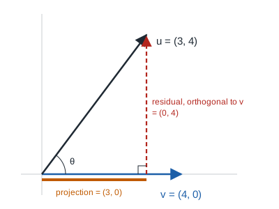
What’s left, $u - \mathrm{proj}_v(u)$ , is orthogonal to $v$ . In the figure, with $u = (3, 4)$ and $v = (4, 0)$ , the projection is $(3, 0)$ and the residual $(0, 4)$ is indeed vertical. We’ll see this “explained part + orthogonal residual” split again in least squares (M2) and PCA (M3).

Where it shows up in ML:

• Linear model: $\hat y = w^\top x + b$ is a dot product. The model measures how aligned example $x$ is with direction $w$ (part 16).
• Neuron: each neuron computes $w^\top x + b$ before its activation (part 21).
• Attention: the score between a query $q$ and a key $k$ is $q^\top k$ (part 23).

3. Norms: measuring length

Intuition. A norm measures a vector’s “size”. There are several sensible ways to do it, depending on what you want to penalize.

$$\begin{aligned} \|x\|_1 &= \sum_i |x_i| \\ \|x\|_2 &= \sqrt{\sum_i x_i^2} = \sqrt{\langle x, x \rangle} \\ \|x\|_\infty &= \max_i |x_i| \end{aligned}$$

• $L_2$ (Euclidean): the straight-line length. It heavily penalizes large components, because of the square.
• $L_1$ (Manhattan): the distance moving only along the axes, like on a city grid. Every component counts proportionally.
• $L_\infty$ : only the largest component counts.

Example: for $u = (3, 4)$ , $\|u\|_2 = 5$ , $\|u\|_1 = 7$ and $\|u\|_\infty = 4$ .

Unit balls. The set of points with norm 1 has a different shape for each norm: a diamond for $L_1$ , a circle for $L_2$ , a square for $L_\infty$ .

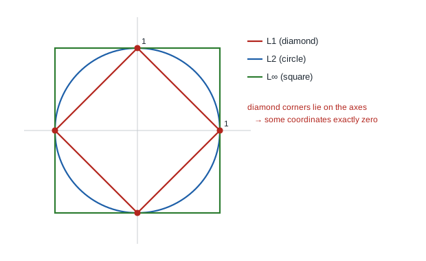
This isn’t cosmetic: the diamond’s corners lie on the axes, where some coordinates are exactly zero. That’s why $L_1$ regularization (Lasso) sets weights to zero and selects features, while $L_2$ (Ridge) shrinks them without zeroing them. The full argument comes in M11, and we’ll use it in part 16.

4. Euclidean distance or cosine similarity?

Intuition. Two different questions: “are these two points close?” and “do these two arrows point the same way?”.

$$\begin{aligned} d(u, v) &= \|u - v\|_2 \\ \cos(u, v) &= \frac{\langle u, v\rangle}{\|u\|_2\,\|v\|_2} \end{aligned}$$

• Distance is scale-sensitive: a vector and its double are far apart.
• Cosine ignores scale: a vector and its double have cosine 1.

For memory access profiles the difference is fundamental: two regions with the same rhythm but not the same intensity are very different in the Euclidean sense, and identical in the cosine sense. The code below shows it in numbers.

Watch the feature scales. With Euclidean distance, a feature in milliseconds (values around 500) crushes a feature between 0 and 1. That’s why we standardize features before kNN, regularized regression or a neural network (part 14).

---

Code example

Four independent blocks: basic operations, Euclidean vs cosine on access profiles, unit balls, and a hand-written kNN.

Basic operations

import numpy as np

u = np.array([3.0, 4.0])
v = np.array([4.0, 0.0])

print("u + v      =", u + v)
print("2u         =", 2 * u)
print("<u, v>     =", u @ v)                          # dot product
print("||u||_2    =", np.linalg.norm(u))              # 5.0
print("||u||_1    =", np.linalg.norm(u, ord=1))       # 7.0
print("||u||_inf  =", np.linalg.norm(u, ord=np.inf))  # 4.0

cos_theta = (u @ v) / (np.linalg.norm(u) * np.linalg.norm(v))
print("angle(u,v) =", np.degrees(np.arccos(cos_theta)).round(2), "degrees")

# projection of u onto the direction of v
proj = (u @ v) / (v @ v) * v
print("proj_v(u)  =", proj, "| residual:", u - proj, "| <residual, v> =", (u - proj) @ v)

The angle is 53.13°, the projection of $u$ onto $v$ is $(3, 0)$ , and the residual $(0, 4)$ is indeed orthogonal to $v$ : their dot product is zero.

Euclidean vs cosine, on access profiles

Each region is described by its accesses over the last 20 aggregations: a vector in $\mathbb{R}^{20}$ .

import numpy as np

t = np.arange(20)
pattern = ((t % 5) < 2).astype(float)       # active 2 aggregations out of 5

profiles = {
    "A: periodic, light":    2 * pattern,
    "B: periodic, intense":  8 * pattern,              # same rhythm, 4x more accesses
    "C: hot, steady":        np.full(20, 3.0),
    "D: periodic, shifted":  2 * np.roll(pattern, 2),  # same intensity as A, out of phase
}
names = list(profiles)
X = np.array([profiles[n] for n in names])


def euclid(a, b):
    return np.linalg.norm(a - b)


def cosine(a, b):
    return (a @ b) / (np.linalg.norm(a) * np.linalg.norm(b))


print("Euclidean distance / cosine similarity to A:")
for n, x in zip(names[1:], X[1:]):
    print(f"  {n:<22} euclid = {euclid(X[0], x):6.2f} | cosine = {cosine(X[0], x):.3f}")

Compared to A	Euclidean distance	Cosine
B: same rhythm, 4× more intense	16.97 (furthest)	1.000 (identical)
C: hot, steady	10.77	0.632
D: same rhythm, shifted by 2 steps	8.00 (closest)	0.000 (orthogonal)

Two key observations:

• by Euclidean distance, the shifted region D is closer to A than B, which has exactly the same rhythm. Intensity dominates everything;
• cosine sees that A and B share the same pattern, but finds D orthogonal to A: the two regions are never active at the same instants. Neither measure captures that D has A’s rhythm, up to a shift.

That’s exactly why in part 14 we don’t compare raw profiles: we build shift-invariant features such as periode_estimee and phase. The tool that measures how much a signal resembles a shifted copy of itself is autocorrelation (M7).

Unit balls

This script reproduces the figure from section 3.

import numpy as np
import matplotlib.pyplot as plt

theta = np.linspace(0, 2 * np.pi, 400)
directions = np.stack([np.cos(theta), np.sin(theta)], axis=1)

fig, ax = plt.subplots(figsize=(5, 5))
for p, name in [(1, "$L_1$"), (2, "$L_2$"), (np.inf, "$L_\\infty$")]:
    norms = np.linalg.norm(directions, ord=p, axis=1)
    pts = directions / norms[:, None]         # rescale each direction to norm 1
    ax.plot(pts[:, 0], pts[:, 1], label=name)
ax.set_aspect("equal")
ax.axhline(0, c="gray", lw=0.5)
ax.axvline(0, c="gray", lw=0.5)
ax.legend()
ax.set_title("Unit balls: $\\{x : \\|x\\|_p = 1\\}$")
plt.show()

The trick: take directions at every angle, then divide each by its $p$ -norm. You get the diamond, the circle and the square.

k-nearest neighbors, by hand

kNN is the most directly geometric algorithm: to classify a point, take the majority class of its $k$ nearest neighbors. Everything therefore hinges on the chosen distance.

We classify periodic profiles (class 1) against random ones (class 0), with widely varying intensities, from 0.5 to 10.

import numpy as np

rng = np.random.default_rng(0)


def knn_predict(X_train, y_train, x, k=5, distance="l2"):
    if distance == "l2":
        d = np.linalg.norm(X_train - x, axis=1)
    elif distance == "l1":
        d = np.abs(X_train - x).sum(axis=1)
    elif distance == "cosine":
        d = 1 - (X_train @ x) / (np.linalg.norm(X_train, axis=1) * np.linalg.norm(x) + 1e-12)
    else:
        raise ValueError(distance)
    neighbors = np.argsort(d)[:k]
    return np.bincount(y_train[neighbors]).argmax()


def generate(n, rng):
    """Periodic (1) or random (0) profiles with varied intensities."""
    Xs, ys = [], []
    for _ in range(n):
        intensity = rng.uniform(0.5, 10)
        if rng.random() < 0.5:
            period = rng.integers(3, 7)
            x = ((np.arange(20) + rng.integers(0, period)) % period == 0) * intensity
            ys.append(1)
        else:
            x = (rng.random(20) < 0.25) * intensity
            ys.append(0)
        Xs.append(x + rng.normal(0, 0.1, 20))
    return np.array(Xs), np.array(ys)


X_tr, y_tr = generate(400, rng)
X_te, y_te = generate(200, rng)
for dist in ("l2", "l1", "cosine"):
    preds = np.array([knn_predict(X_tr, y_tr, x, k=5, distance=dist) for x in X_te])
    print(f"kNN distance {dist:<7} accuracy = {np.mean(preds == y_te):.3f}")

Distance	Accuracy
$L_2$	0.745
$L_1$	0.745
cosine	0.860

Cosine wins clearly, because the class depends on the profile’s shape, not its intensity. With $L_1$ or $L_2$ , an intense periodic profile looks more like an intense random one than a light periodic one. Choosing a distance is a modeling choice: it encodes what you consider “similar”.

---

Hands-on exercise

1. By hand. For $u = (1, 2, 2)$ and $v = (2, 0, -1)$ , compute $\|u\|_1$ , $\|u\|_2$ , $\|u\|_\infty$ , $\langle u, v\rangle$ and the angle between $u$ and $v$ . Check with NumPy.
2. Cauchy-Schwarz inequality. Draw 10,000 random vector pairs in $\mathbb{R}^{10}$ and check numerically that $|\langle u, v\rangle| \le \|u\|_2\|v\|_2$ . Using the geometric definition, explain why it always holds and when equality occurs.
3. Normalize to reconcile. In the kNN, divide each vector by its $L_2$ norm (for X_tr and X_te) before using the $L_2$ distance. What happens to accuracy? Show that for unit vectors, $\|u - v\|_2^2 = 2 - 2\cos(u, v)$ .
4. Shift invariance. Write a function computing the maximum cosine between $a$ and every shifted version of $b$ (np.roll(b, s) for $s = 0, \dots, 19$ ). Check that it finally sees A and D as similar. Then plug it into the kNN: does accuracy improve?
5. Running project. In the part 14 traces, which feature would be dominated by the others under Euclidean distance without standardization? Look at the scales of depuis_dernier (up to 500) and frac_active_20 (between 0 and 1).

Hint for question 3: expand $\|u - v\|^2 = \langle u - v, u - v\rangle$ using the bilinearity of the dot product.

---

Further resources

• 3Blue1Brown, Essence of Linear Algebra, episodes 1, 2 and 9 (Dot products and duality): the visual intuition, on video.
• Deisenroth, Faisal, Ong, Mathematics for Machine Learning, chapter 3 (analytic geometry), free online.
• Gilbert Strang, Introduction to Linear Algebra, chapter 1.
• On this blog: NumPy: thinking in arrays, for vectorized computation.

---

What you should be able to do before moving on

• Compute $L_1$ , $L_2$ , $L_\infty$ norms and dot products by hand
• Read a dot product as a measure of alignment and a projection
• Sketch the $L_1$ , $L_2$ , $L_\infty$ unit balls from memory, and say where the diamond’s corners are
• Choose between Euclidean distance and cosine depending on whether intensity matters
• Explain why features are standardized before a distance-based algorithm
• Spot a dot product in $\hat y = w^\top x + b$

Next part: M2 · Matrices as transformations. A matrix applies a transformation to vectors, and a neural network layer is nothing more than that.