M6 · Hessian, convexity and Taylor expansion

Mastering AI · Required Maths · Week 2 (calculus) · Part 6

Goal of this step

The gradient (M4) says which way to go down. It doesn’t say how far you can go without overshooting, nor whether the bottom of the valley is unique. Both come from curvature, measured by the second derivative and, in several dimensions, by the Hessian matrix.

By the end of this article you’ll be able to:

• approximate a function with a first- or second-order Taylor polynomial, and estimate the error;
• compute and interpret a Hessian through its eigenvalues;
• recognize a convex function, and show that the log-loss is one;
• explain conditioning, the maximum gradient descent step and Newton’s method;
• recognize a saddle point.

---

Key concepts

1. Taylor expansion

Intuition. Near a point, a smooth function looks like a line (first order, M4’s tangent). To do better, add a curvature term: it then looks like a parabola (second order).

In one variable, around $x_0$ :

$$f(x_0 + h) = f(x_0) + f'(x_0)\,h + \tfrac{1}{2} f''(x_0)\,h^2 + O(h^3)$$

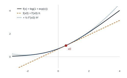
The first-order error is proportional to $h^2$ , the second-order one to $h^3$ . Halving $h$ divides the first error by 4 and the second by 8. That’s what explains the centered difference’s advantage in M4: its $h^2$ terms cancel.

In several variables, the first-order term is a dot product with the gradient, and the second-order term involves the Hessian $H$ :

$$f(w + h) \approx f(w) + \nabla f(w)^\top h + \tfrac{1}{2}\, h^\top H(w)\, h$$

2. The Hessian: curvature in every direction

Intuition. The gradient gives the slope in each direction. The Hessian gives the curvature in each direction: does the slope steepen (valley), flatten (peak), or both depending on the direction (pass)?

$$H_{ij} = \frac{\partial^2 f}{\partial w_i \, \partial w_j}$$

For a smooth function, $H$ is symmetric. M3’s spectral theorem applies: $H$ has real eigenvalues and orthogonal eigen-directions. Each eigenvalue $\lambda_i$ is the curvature along its eigen-direction:

• $\lambda_i > 0$ : the function rises on both sides, like a valley;
• $\lambda_i < 0$ : it falls on both sides, like a peak;
• $\lambda_i = 0$ : it’s flat, at least to second order.

Example: for the quadratic $q(w) = \frac{1}{2} w^\top A w$ , the Hessian is simply $A$ .

3. Convexity

Intuition. A convex function is bowl-shaped: the segment between two points of the graph always stays above the graph. Crucial consequence: every local minimum is a global minimum. Descent can’t get stuck in a bad dip.

Practical test: a twice-differentiable function is convex if and only if its Hessian is positive semi-definite everywhere, i.e. all its eigenvalues are $\geq 0$ , or $h^\top H h \geq 0$ for every $h$ .

The log-loss is convex. Its Hessian is:

$$H(w) = \frac{1}{n} X^\top D X, \qquad D = \operatorname{diag}\big(p_i (1 - p_i)\big)$$

For any vector $h$ , $h^\top H h = \frac{1}{n} \sum_i p_i(1 - p_i)\,(x_i^\top h)^2 \geq 0$ , since each term is a positive weight times a square. Logistic regression therefore has a single dip: we’re sure to find the best model. Linear regression’s MSE is convex too ( $H = \frac{2}{n}X^\top X$ ).

A neural network isn’t convex. Simple example: swapping two hidden neurons gives exactly the same network, hence the same loss. There are several distinct minima, which a strictly convex function can’t have.

4. Saddle points

Intuition. A mountain pass: following the road, you’re at the highest point; looking at the peaks on either side, you’re at the lowest. The gradient is zero there, but it’s neither a minimum nor a maximum.

For $f(x, y) = x^2 - y^2$ , the Hessian at $(0, 0)$ has eigenvalues $+2$ and $-2$ . In high dimensions, saddle points vastly outnumber local minima: one reason networks train better than feared.

5. Conditioning and step size

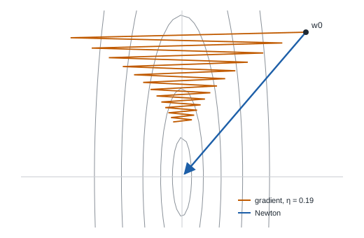
Intuition. If the valley is very steep in one direction and nearly flat in another, a step large enough to make progress in the flat direction makes you bounce in the steep one. You zigzag.

The condition number $\kappa = \lambda_{\max} / \lambda_{\min}$ measures that gap. For gradient descent $w \leftarrow w - \eta \nabla f(w)$ on a quadratic, the Hessian shows that:

• it only converges if $\eta < 2 / \lambda_{\max}$ ;
• with the best step, the error shrinks by a factor of about $\frac{\kappa - 1}{\kappa + 1}$ per iteration: very slowly if $\kappa$ is large.

That’s why we standardize features (M1, part 14): features on very different scales give an ill-conditioned Hessian.

6. Newton’s method

Intuition. Instead of following the slope, replace the function with its second-order Taylor parabola and jump straight to the bottom of that parabola. Setting the approximation’s gradient to zero gives:

$$w \leftarrow w - H(w)^{-1} \nabla f(w)$$

On a quadratic, Newton reaches the minimum in one step, whatever $\kappa$ . On the log-loss, it converges in a few iterations. Its price: storing and solving a system with the $d \times d$ Hessian. Fine for 9 features, impossible for a network with a million weights. That’s why deep learning uses smarter first-order methods (momentum, Adam, M10), which partly mimic the effect of curvature.

---

Code example

Taylor: errors in $h^2$ and $h^3$

import numpy as np

f = lambda x: np.log(1 + np.exp(x))            # softplus
f1 = lambda x: 1 / (1 + np.exp(-x))            # f'  = sigmoid
f2 = lambda x: f1(x) * (1 - f1(x))             # f'' = σ(1 − σ)
x0 = 0.5
print("h        order-1 error     order-2 error")
for h in (0.5, 0.25, 0.125, 0.0625):
    t1 = f(x0) + f1(x0) * h
    t2 = t1 + 0.5 * f2(x0) * h**2
    print(f"{h:<8} {abs(f(x0 + h) - t1):.2e}          {abs(f(x0 + h) - t2):.2e}")

$h$	Order-1 error	Order-2 error
0.5	$2.80 \times 10^{-2}$	$1.42 \times 10^{-3}$
0.25	$7.18 \times 10^{-3}$	$1.65 \times 10^{-4}$
0.125	$1.82 \times 10^{-3}$	$1.97 \times 10^{-5}$
0.0625	$4.57 \times 10^{-4}$	$2.40 \times 10^{-6}$

Halving $h$ divides the order-1 error by about 4 and the order-2 error by about 8: $h^2$ and $h^3$ , as predicted.

Conditioning, maximum step and Newton

import numpy as np

A = np.array([[10.0, 0.0], [0.0, 0.2]])        # very different curvatures along the axes
q = lambda w: 0.5 * w @ A @ w
grad_q = lambda w: A @ w
vals = np.linalg.eigvalsh(A)
print("Hessian eigenvalues:", vals, "| condition number κ =", vals.max() / vals.min())


def descent(w, eta, n_iter):
    path = [w.copy()]
    for _ in range(n_iter):
        w = w - eta * grad_q(w)
        path.append(w.copy())
    return np.array(path)


w0 = np.array([1.0, 2.0])
for eta in (0.05, 0.19, 0.21):
    path = descent(w0, eta, 100)
    print(f"descent η={eta}: q after 100 iterations = {q(path[-1]):.2e}")
newton = w0 - np.linalg.solve(A, grad_q(w0))
print("Newton, 1 iteration:", newton, "| q =", q(newton))

Method	$q$ after 100 iterations
gradient, $\eta = 0.05$	$5.4 \times 10^{-2}$
gradient, $\eta = 0.19$	$1.7 \times 10^{-4}$
gradient, $\eta = 0.21$	$9.5 \times 10^{8}$ (diverges)
Newton, 1 iteration	$0$

With $\lambda_{\max} = 10$ , the theoretical limit is $\eta < 2/10 = 0.2$ . At $0.19$ it converges while zigzagging; at $0.21$ it blows up. A cautious step ( $0.05$ ) avoids bouncing but barely moves along the flat direction ( $\lambda = 0.2$ ).

The log-loss is convex, and Newton shines on it

We reuse M4’s data and compute the Hessian $\frac{1}{n}X^\top D X$ .

import numpy as np

rng = np.random.default_rng(0)
n, d = 500, 3
X = rng.normal(size=(n, d))
sig = lambda z: 1 / (1 + np.exp(-z))
y = (rng.random(n) < sig(X @ np.array([1.5, -2.0, 0.5]))).astype(float)
loss = lambda w: -np.mean(y * np.log(sig(X @ w)) + (1 - y) * np.log(1 - sig(X @ w)))
grad = lambda w: X.T @ (sig(X @ w) - y) / n
hess = lambda w: (X.T * (sig(X @ w) * (1 - sig(X @ w)))) @ X / n

for _ in range(3):
    w = rng.normal(size=d) * 3
    print("eigenvalues of H at a random w:", np.linalg.eigvalsh(hess(w)).round(4))

# Newton vs gradient descent
w_n, w_g = np.zeros(d), np.zeros(d)
for k in range(1, 201):
    w_n = w_n - np.linalg.solve(hess(w_n), grad(w_n)) if k <= 8 else w_n
    w_g = w_g - 1.0 * grad(w_g)
    if k in (1, 2, 3, 5, 8, 50, 200):
        print(f"iteration {k:>3} | Newton: {loss(w_n):.6f} | gradient: {loss(w_g):.6f}")

At three random points, all eigenvalues of $H$ are positive (for example $0.004$ , $0.056$ and $0.063$ ): the log-loss is indeed convex.

Iteration	Newton	Gradient descent
1	0.486768	0.618094
3	0.463187	0.544190
5	0.463175	0.511440
50	0.463175	0.463258
200	0.463175	0.463175

Newton reaches the optimum to six decimals in 5 iterations; gradient descent takes 200. Each Newton iteration costs more (a $3 \times 3$ Hessian to build and a system to solve), but with 3 parameters that’s negligible.

---

Hands-on exercise

1. Taylor by hand. Write the second-order expansions of $e^x$ and $\ln(1 + x)$ around 0. For $x = 0.1$ , compare the approximations with the true values.
2. Hessian of a saddle. Compute by hand the Hessian of $f(x, y) = x^3 - 3xy^2$ (the “monkey saddle”). What are its eigenvalues at $(0, 0)$ ? At $(1, 0)$ ?
3. The maximum step. For $A = \operatorname{diag}(4, 1)$ , predict gradient descent’s maximum step, then check by trying $\eta = 0.49$ and $\eta = 0.51$ .
4. Standardizing improves conditioning. Build a matrix $X$ with 2 features, one in milliseconds (values around 500), the other between 0 and 1. Compute the condition number of $X^\top X$ before and after StandardScaler. Relate it to gradient descent speed.
5. Running project. For a logistic regression on 9 features, the Hessian is $9 \times 9$ . Is Newton reasonable? That’s in fact what scikit-learn’s newton-cg solver does. What about an LSTM with 50,000 weights?

Hint for question 3: the limit is $2/\lambda_{\max}$ .

---

Further resources

• Boyd and Vandenberghe, Convex Optimization, chapter 3 (convex functions) and section 9.5 (Newton’s method), free online.
• Deisenroth et al., Mathematics for Machine Learning, sections 5.8 (Taylor) and 7.3 (convex optimization).
• Dauphin et al., Identifying and attacking the saddle point problem in high-dimensional non-convex optimization (NeurIPS 2014).
• Distill, Why Momentum Really Works: conditioning in interactive pictures (we’ll come back to it in M10).

---

What you should be able to do before moving on

• Write a second-order Taylor expansion, in one and several variables
• Compute a Hessian and read its eigenvalues as curvatures
• Recognize a convex function and show that the log-loss is one
• Tell a minimum, a maximum and a saddle point apart with the Hessian
• Explain conditioning and the maximum step $2/\lambda_{\max}$
• Explain why Newton converges fast and why it isn’t used for large networks

Next part: M7 · Random variables, distributions, expectation and variance. Probability week starts: the minimal vocabulary for reasoning under uncertainty.