October 16, 2026 · 21 min read

M10 · Gradient descent and its variants

SGD, momentum, Adam and gradient boosting: how a loss is actually minimized, and why the learning rate matters so much.

Mastering AI · Required Maths · Week 4 (optimization) · Part 10

Goal of this step

Since M4 you know how to compute a gradient, and since M5 how to get it for free with backpropagation. Now you have to use it: start from a random point and walk down to the bottom of the loss. That is what every fit() you’ve called does behind the scenes, from logistic regression to the LSTM in the thesis.

By the end of this article you’ll be able to:

write the gradient descent update and justify it with Taylor (M6);
explain why the learning rate decides everything, and recognize a step that is too small, too large, or “just a bit too large”;
explain what stochastic and mini-batch gradients bring, and why their noise forces you to lower the learning rate;
write momentum, RMSProp and Adam from memory, and say what each one fixes;
see gradient boosting as gradient descent in a space of functions;
implement all of this in NumPy and check your Adam against torch.optim.Adam.

Key concepts

1. Gradient descent

Intuition. You’re on a mountain in the fog. You can’t see the valley, only the slope under your feet. The gradient points uphill (M4): take a small step the other way, and start again.

$\theta_{t+1} = \theta_t - \eta\,\nabla L(\theta_t)$

$\eta > 0$ is the learning rate. Why does it work? The second-order Taylor expansion (M6), with $g = \nabla L(\theta_t)$ and $H$ the Hessian, gives:

$L(\theta_t - \eta g) \approx L(\theta_t) - \eta\,\lVert g \rVert^2 + \frac{\eta^2}{2}\, g^\top H g$

The second term always lowers the loss; the third one, due to curvature, raises it again. For a small enough $\eta$ , the linear term wins and the loss goes down. Since $g^\top H g \le \lambda_{\max} \lVert g \rVert^2$ , a step $\eta < 2/\lambda_{\max}$ is enough to guarantee the decrease on a quadratic: that’s M6’s maximum step.

2. The learning rate: the most important hyperparameter

Intuition. Too small, you crawl. Too large, you bounce from one wall of the valley to the other, or you’re thrown out of it.

M6 gave the two key results on a quadratic with condition number $\kappa = \lambda_{\max}/\lambda_{\min}$ :

convergence only if $\eta < 2/\lambda_{\max}$ ;
even with the best step, the error only shrinks by a factor $\frac{\kappa - 1}{\kappa + 1}$ per iteration.

On a non-convex function, $\lambda_{\max}$ is the local curvature, which changes along the way. Take the Rosenbrock function, a classic optimization benchmark:

$f(x, y) = (1 - x)^2 + 100\,(y - x^2)^2$

Its minimum is at $(1, 1)$ , at the bottom of a curved, narrow valley. There, the Hessian has eigenvalues $1001.6$ and $0.40$ : $\kappa \approx 2{,}500$ , and the maximum step is $2/1001.6 \approx 0.0020$ . We’ll see that with $\eta = 0.0021$ , just 5% too large, descent never reaches the minimum: it ends up bouncing on the walls.

That’s also why we standardize features (part 14): features on very different scales give an ill-conditioned Hessian, so a tiny maximum step and a crawling descent in the flat directions. We measure it on the running project below.

3. Stochastic and mini-batch gradients

Intuition. The loss is a mean over $n$ examples, so its gradient is too. To decide which way to go, there’s no need to poll all $n$ examples: a random sample of $B$ of them gives a good estimate, $n/B$ times cheaper.

$\nabla L(\theta) = \frac{1}{n}\sum_{i=1}^{n} \nabla \ell_i(\theta) \qquad \hat g_B = \frac{1}{B}\sum_{i \in \mathcal{B}} \nabla \ell_i(\theta)$

With a mini-batch $\mathcal{B}$ drawn at random, $\hat g_B$ is an unbiased estimator of the true gradient (M7: its expectation is $\nabla L$ ), and its variance shrinks as $\sigma^2/B$ (M9: the standard error decays as $1/\sqrt B$ ).

Full-batch gradient descent ( $B = n$ ): one precise step per pass over the data (an epoch).
SGD ( $B = 1$ ) and mini-batch ( $B = 32$ to $512$ typically): many approximate steps per epoch. On large datasets, that’s much faster to get close to the minimum.

The price: with a constant $\eta$ , the noise never vanishes. Close to the minimum, the true gradient tends to 0 but $\hat g_B$ doesn’t: you jiggle around the minimum at a distance that grows with $\eta$ and shrinks with $B$ . Two remedies: decrease $\eta$ over time (a schedule: step decay, cosine, linear warm-up then decay), or increase $B$ . The classic theory (Robbins and Monro, 1951) asks for $\sum_t \eta_t = \infty$ (go far enough) and $\sum_t \eta_t^2 < \infty$ (end up stopping).

This noise also has a virtue: it helps you leave saddle points (M6) and flat areas, where the exact gradient is almost zero.

4. Momentum

Intuition. A ball rolling down a valley picks up speed in the direction where the slope is consistent, and its inertia cancels out the back-and-forth from one wall to the other.

\begin{aligned} v_{t+1} &= \beta\, v_t + \nabla L(\theta_t) \\ \theta_{t+1} &= \theta_t - \eta\, v_{t+1} \end{aligned}

$v$ is an accumulation of past gradients, with forgetting factor $\beta$ (typically $0.9$ ). If the gradient keeps pointing the same way, $v$ grows up to $g/(1 - \beta)$ : the effective step is $\eta/(1 - \beta)$ , i.e. 10 times bigger with $\beta = 0.9$ . If it flips sign at every step (the zigzag of an ill-conditioned valley), the contributions cancel. Momentum therefore speeds up the flat directions without blowing up the steep ones. On a quadratic, the right choice of $\eta$ and $\beta$ brings the factor $\frac{\kappa - 1}{\kappa + 1}$ down to $\frac{\sqrt\kappa - 1}{\sqrt\kappa + 1}$ : with $\kappa = 2{,}500$ , that’s 0.96 per step instead of 0.9992.

Nesterov’s variant computes the gradient at the point where momentum is about to take you, $\theta_t - \eta\beta v_t$ , rather than at $\theta_t$ : it anticipates the turn a little.

5. RMSProp and Adam: one step per coordinate

Intuition. One learning rate for all parameters is a poor compromise when gradients have very different scales from one coordinate to another. Idea: divide each coordinate by the typical size of its recent gradients. Coordinates with big gradients get slowed down, the timid ones get a push.

RMSProp (Hinton, 2012) keeps a moving average of squared gradients and divides by its square root. Adam (Kingma and Ba, 2015) adds momentum to it:

\begin{aligned} m_t &= \beta_1\, m_{t-1} + (1 - \beta_1)\, g_t \\ v_t &= \beta_2\, v_{t-1} + (1 - \beta_2)\, g_t^2 \\ \hat m_t &= \frac{m_t}{1 - \beta_1^t}, \qquad \hat v_t = \frac{v_t}{1 - \beta_2^t} \\ \theta_t &= \theta_{t-1} - \eta\, \frac{\hat m_t}{\sqrt{\hat v_t} + \varepsilon} \end{aligned}

with, by default, $\beta_1 = 0.9$ , $\beta_2 = 0.999$ , $\varepsilon = 10^{-8}$ ; operations on vectors are element-wise.

$m_t$ is momentum (average of gradients), $v_t$ the average of their squares (an estimate of their scale).
$\hat m_t$ and $\hat v_t$ correct the bias from initializing at 0: at $t = 1$ , $m_1 = 0.1\,g_1$ would otherwise be 10 times too small.
The ratio $\hat m_t / \sqrt{\hat v_t}$ is roughly between $-1$ and $1$ : each coordinate moves by about $\eta$ per step, whatever the scale of its gradient. That makes Adam far less sensitive to poorly scaled features, and $\eta = 10^{-3}$ is a reasonable default almost everywhere.

The flip side: since the step stays close to $\eta$ even when the gradient becomes tiny, Adam with a constant $\eta$ doesn’t settle down neatly at the minimum. You’ll see it on the figure below. In practice it’s paired with a decreasing schedule. And to regularize, use AdamW, which applies weight decay outside the $\sqrt{\hat v_t}$ normalization (M11).

6. Gradient boosting: a gradient descent on functions

Intuition. Instead of moving a parameter vector $\theta$ , you move the predictions themselves. At each step, you compute in which direction each prediction should move to lower the loss, then fit a small tree that approximately points that way.

Write $F(x)$ for the model’s score (the log-odds, for classification). The loss depends on the $n$ values $F(x_i)$ ; its gradient with respect to these values is computed example by example. For the log-loss (M8), with $p_i = \sigma(F(x_i))$ :

$-\frac{\partial \ell_i}{\partial F(x_i)} = y_i - p_i$

The negative gradient is just the residual “label minus predicted probability”. Gradient boosting then does:

$F_m = F_{m-1} + \nu\, h_m, \qquad h_m \approx \argmin_{h \in \text{trees}} \sum_{i=1}^{n} \big(r_i - h(x_i)\big)^2, \quad r_i = y_i - p_i$

$\nu$ (the learning_rate of LightGBM and XGBoost) plays exactly the role of $\eta$ . The difference from section 1: you can’t move each $F(x_i)$ freely (that would be learning the training set by heart), so the step is projected onto what a small tree can represent, which generalizes to new examples.

LightGBM goes one step further: it uses the gradient and the second derivative $p_i(1 - p_i)$ to compute each leaf’s value, $-\sum g_i / (\sum h_i + \lambda)$ . That’s a Newton step (M6) per leaf: it converges much faster than plain residuals, as you’ll see in exercise 5.

Code example

GD, momentum, Adam and noisy SGD on Rosenbrock

Every optimizer is written with the same signature: it receives the gradient, the position, the step and its internal state, and returns the new position and the new state.

import numpy as np


def rosenbrock(p):
    x, y = p
    return (1 - x) ** 2 + 100 * (y - x ** 2) ** 2


def grad_rosenbrock(p):
    x, y = p
    return np.array([-2 * (1 - x) - 400 * x * (y - x ** 2), 200 * (y - x ** 2)])


def sgd(g, p, eta, state, t):
    return p - eta * g, None


def momentum(g, p, eta, state, t, beta=0.9):
    v = g if state is None else beta * state + g        # velocity: sum of past gradients
    return p - eta * v, v


def adam(g, p, eta, state, t, b1=0.9, b2=0.999, eps=1e-8):
    m, v = (np.zeros_like(p), np.zeros_like(p)) if state is None else state
    m = b1 * m + (1 - b1) * g                           # moving average of gradients
    v = b2 * v + (1 - b2) * g ** 2                      # moving average of squared gradients
    m_hat, v_hat = m / (1 - b1 ** t), v / (1 - b2 ** t) # bias correction
    return p - eta * m_hat / (np.sqrt(v_hat) + eps), (m, v)


def run(step, eta, n_steps=20_000, noise=0.0, seed=0):
    """Optimize from (-1.2, 1). noise > 0 simulates a stochastic gradient."""
    rng = np.random.default_rng(seed)
    p, state, path = np.array([-1.2, 1.0]), None, []
    for t in range(1, n_steps + 1):
        g = grad_rosenbrock(p) + noise * rng.normal(size=2)
        p, state = step(g, p, eta, state, t)
        path.append(p.copy())
    return np.array(path)


runs = {
    "GD, eta = 0.001": run(sgd, 1e-3),
    "GD, eta = 0.0021": run(sgd, 2.1e-3),
    "momentum 0.9, eta = 0.001": run(momentum, 1e-3),
    "Adam, eta = 0.01": run(adam, 1e-2),
    "noisy SGD, eta = 0.001": run(sgd, 1e-3, noise=10.0),
}
for name, path in runs.items():
    dist = np.linalg.norm(path - 1.0, axis=1)          # distance to the minimum (1, 1)
    first = int(np.argmax(dist < 1e-3)) + 1 if (dist < 1e-3).any() else "never"
    print(f"{name:<26} f(θ_20000) = {rosenbrock(path[-1]):.1e} | first step at < 1e-3: {first:>5} | "
          f"mean distance (last 1,000 steps) = {dist[-1000:].mean():.1e}")

After 20,000 steps from $(-1.2, 1)$ :

Optimizer	$f$ after 20,000 steps	First step within $10^{-3}$ of the minimum	Mean distance over the last 1,000 steps
GD, $\eta = 0.001$	$1.9 \times 10^{-8}$	17,082	$3.8 \times 10^{-4}$
GD, $\eta = 0.0021$	$4.0 \times 10^{-2}$	never	$7.0 \times 10^{-2}$
Momentum 0.9, $\eta = 0.001$	$2.0 \times 10^{-30}$	1,580	$2.1 \times 10^{-15}$
Adam, $\eta = 0.01$	$5.0 \times 10^{-11}$	4,409	$1.7 \times 10^{-4}$
Noisy SGD, $\eta = 0.001$	$1.8 \times 10^{-2}$	13,180 (by chance)	$1.1 \times 10^{-1}$

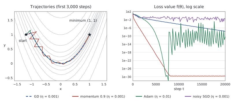
What to take away:

Plain GD finds the valley quickly, then crawls along it: it takes 17,082 steps to get within $10^{-3}$ of the minimum. That’s the flat direction ( $\lambda = 0.40$ ) we can’t speed up without blowing up the steep one ( $\lambda = 1001.6$ ).
5% too large is enough to fail. With $\eta = 0.0021 > 2/1001.6$ , GD never converges: at the bottom of the valley it bounces on the walls and stays stuck at $f = 0.04$ . Nothing diverges spectacularly: it’s a silent failure, the kind you only see by plotting the loss.
Momentum zigzags at first (the left figure), then its accumulated velocity carries it along the valley: within $10^{-3}$ in 1,580 steps, more than 10 times faster than GD with the same $\eta$ , and down to machine precision afterwards.
Adam gets close in 4,409 steps, then oscillates: the right curve shows peaks between $10^{-16}$ and $10^{-3}$ . Near the minimum, gradients become tiny, $\hat v_t$ follows slowly (memory of 1,000 steps), and the ratio $\hat m_t/\sqrt{\hat v_t}$ makes it take steps of size about $\eta$ again. Hence the need for a decreasing schedule.
Noisy SGD (Gaussian noise of standard deviation 10 added to the gradient) goes down the valley but stays at an average distance of 0.11 from the minimum: that’s the noise floor of a constant learning rate. It passed within $10^{-3}$ once at step 13,180, by chance, without staying there.

Running project: training a logistic regression by hand

We take M9’s synthetic memory regions and the logistic regression with domain features (log of accesses, “periodic and peak imminent” interaction). This time we train it ourselves, comparing optimizers at equal number of epochs (passes over the 3,500 training regions), which is the fair measure of compute cost.

import numpy as np
from sklearn.linear_model import LogisticRegression
from sklearn.metrics import log_loss
from sklearn.model_selection import train_test_split


def make_regions(n, rng):
    """Synthetic memory regions (same generator as M9): label 1 = hot in the next window."""
    rate = rng.gamma(0.6, 4, n)
    recent_accesses = rng.poisson(rate)
    since_last = np.round(rng.exponential(30 / (1 + recent_accesses)), 1)
    periodic = rng.binomial(1, 0.25, n)
    before_peak = rng.integers(0, 12, n)
    logit = (0.9 * np.log1p(recent_accesses) - 0.05 * since_last
             + 3.0 * periodic * (before_peak < 3) - 1.5 + rng.normal(0, 0.8, n))
    X = np.column_stack([recent_accesses, since_last, periodic, before_peak])
    return X, (logit > 0).astype(int)


def domain_features(X):
    return np.column_stack([np.log1p(X[:, 0]), X[:, 1], X[:, 2], X[:, 2] * (X[:, 3] < 3)])


rng = np.random.default_rng(0)
X, y = make_regions(5000, rng)
Xtr, Xte, ytr, yte = train_test_split(X, y, test_size=0.3, random_state=0, stratify=y)
Ftr = domain_features(Xtr)
Ztr = (Ftr - Ftr.mean(axis=0)) / Ftr.std(axis=0)          # standardized features
A_raw = np.column_stack([np.ones(len(Ftr)), Ftr])         # column of 1s = intercept
A_std = np.column_stack([np.ones(len(Ztr)), Ztr])


def loss_grad(w, A, y):
    """Mean log loss of a logistic regression (M8) and its gradient."""
    p = np.clip(1 / (1 + np.exp(-(A @ w))), 1e-12, 1 - 1e-12)
    return -np.mean(y * np.log(p) + (1 - y) * np.log(1 - p)), A.T @ (p - y) / len(y)


# reference optimum (no regularization)
ref = LogisticRegression(C=np.inf, max_iter=10_000, tol=1e-10).fit(Ztr, ytr)
L_star = log_loss(ytr, ref.predict_proba(Ztr)[:, 1])
print(f"optimal log loss (sklearn) = {L_star:.4f}")

# conditioning: at w = 0, the Hessian is Aᵀ A / (4n)
for name, A in (("raw", A_raw), ("standardized", A_std)):
    eig = np.linalg.eigvalsh(A.T @ A / (4 * len(A)))
    print(f"{name:<13}: λ_max = {eig[-1]:.3g}, λ_min = {eig[0]:.3g}, condition number = {eig[-1] / eig[0]:.0f}")


def train(A, y, optimizer, eta, epochs=200, batch=None, seed=0):
    """Returns the training log loss (whole set) after each epoch."""
    rng = np.random.default_rng(seed)
    n, w = len(y), np.zeros(A.shape[1])
    m, v, t, history = np.zeros_like(w), np.zeros_like(w), 0, []
    for _ in range(epochs):
        order = rng.permutation(n)
        for start in range(0, n, batch or n):          # batch=None: one step per epoch (full GD)
            i = order[start:start + (batch or n)]
            _, g = loss_grad(w, A[i], y[i])
            t += 1
            if optimizer == "sgd":
                w -= eta * g
            else:                                      # adam
                m = 0.9 * m + 0.1 * g
                v = 0.999 * v + 0.001 * g ** 2
                w -= eta * (m / (1 - 0.9 ** t)) / (np.sqrt(v / (1 - 0.999 ** t)) + 1e-8)
        history.append(loss_grad(w, A, y)[0])
    return np.array(history)


setups = {
    "GD, raw, eta = 0.005": (A_raw, "sgd", 0.005, None),
    "GD, raw, eta = 0.2": (A_raw, "sgd", 0.2, None),
    "GD, standardized, eta = 4": (A_std, "sgd", 4.0, None),
    "SGD b=32, standardized, eta = 0.1": (A_std, "sgd", 0.1, 32),
    "SGD b=32, standardized, eta = 0.3": (A_std, "sgd", 0.3, 32),
    "Adam b=32, raw, eta = 0.003": (A_raw, "adam", 0.003, 32),
    "Adam b=32, standardized, eta = 0.01": (A_std, "adam", 0.01, 32),
}
for name, (A, opt, eta, batch) in setups.items():
    h = train(A, ytr, opt, eta, batch=batch)
    gap = h - L_star
    reached = int(np.argmax(gap < 1e-3)) + 1 if (gap < 1e-3).any() else "never"
    print(f"{name:<36} loss after 1 / 10 / 200 epochs = {h[0]:.4f} / {h[9]:.4f} / {h[-1]:.4f} | "
          f"gap < 0.001 at epoch {reached}")

The optimum computed by scikit-learn is a log-loss of 0.2692. First, conditioning at $w = 0$ :

Features	$\lambda_{\max}$	$\lambda_{\min}$	$\kappa$
raw	204	0.011	18,565
standardized	0.367	0.132	3

The time since the last access goes up to 206 while the other features stay between 0 and 3.5: the Hessian is 18,565 times steeper in one direction than in another. After standardization, $\kappa = 3$ .

Optimizer (200 epochs)	Loss after 1 epoch	after 10	after 200	Within 0.001 of the optimum at epoch
GD, raw, $\eta = 0.005$	0.5288	0.4586	0.4407	never
GD, raw, $\eta = 0.2$	1.5607	0.4348	0.3416	never
GD, standardized, $\eta = 4$	0.3403	0.2799	0.2692	57
SGD $B = 32$ , standardized, $\eta = 0.1$	0.3246	0.2733	0.2693	23
SGD $B = 32$ , standardized, $\eta = 0.3$	0.2853	0.2701	0.2698	10
Adam $B = 32$ , raw, $\eta = 0.003$	0.4255	0.3224	0.2692	54
Adam $B = 32$ , standardized, $\eta = 0.01$	0.3644	0.2715	0.2696	13

Four lessons, all predicted by the theory:

Without standardization, GD is stuck. With $\eta = 0.005 \approx 1/\lambda_{\max}$ , it’s stable but still at 0.44 after 200 epochs. With $\eta = 0.2$ , the first epoch overshoots (loss 1.56); the logistic curvature drops when $p$ moves away from 0.5, so it survives, but it’s still at 0.34. The flat direction ( $\lambda_{\min} = 0.011$ ) barely moves.
Standardizing changes everything: the same GD reaches the optimum in 57 epochs, with a step of 4 that would be absurd on raw features.
Mini-batches are worth it per epoch: SGD with $B = 32$ takes 110 steps per epoch instead of one and gets within 0.001 of the optimum in 10 to 23 epochs. But with $\eta = 0.3$ , it then stays at 0.2698 instead of going down to 0.2692: that’s the noise floor, and the reason for a decreasing schedule (exercise 4).
Adam forgives poor scaling: on raw features, it reaches the optimum (0.2692) where GD stalls, because each coordinate gets its own step. Standardizing remains good practice, but it’s no longer a matter of life and death.

Gradient boosting by hand

We now code functional gradient descent from section 6: each tree fits the residuals $y - p$ , and we take a step $\nu = 0.1$ in its direction.

# continues the previous block (make_regions already defined)
from sklearn.metrics import f1_score
from sklearn.tree import DecisionTreeRegressor

rng = np.random.default_rng(0)
X, y = make_regions(5000, rng)
Xtr, Xte, ytr, yte = train_test_split(X, y, test_size=0.3, random_state=0, stratify=y)

sigmoid = lambda f: 1 / (1 + np.exp(-f))
nu = 0.1                                               # shrinkage = learning rate in function space
F_tr = np.full(len(ytr), np.log(ytr.mean() / (1 - ytr.mean())))   # F_0: constant log-odds
F_te = np.full(len(yte), F_tr[0])
for m in range(1, 201):
    residual = ytr - sigmoid(F_tr)                     # = −∂(log loss)/∂F: the negative gradient
    tree = DecisionTreeRegressor(max_depth=3, random_state=0).fit(Xtr, residual)
    F_tr += nu * tree.predict(Xtr)                     # one gradient step... on a function
    F_te += nu * tree.predict(Xte)
    if m in (1, 10, 50, 200):
        print(f"{m:>3} trees: train log loss = {log_loss(ytr, sigmoid(F_tr)):.4f} | "
              f"test F1 = {f1_score(yte, (F_te > 0).astype(int)):.3f}")

Trees	Train log-loss	Test F1
1	0.5200	0.000
10	0.4708	0.000
50	0.3694	0.404
200	0.2954	0.680

Twenty lines of code, on the raw features, with no feature engineering, and we get a test F1 of 0.680, on par with LightGBM in M9 (0.681 on the same test set). The first 10 trees predict no hot region (F1 = 0): plain residuals are small (less than 1 in absolute value), so with $\nu = 0.1$ the scores move slowly away from the starting log-odds, about $-1.3$ , and stay below the threshold of 0. That’s the slowness of first-order steps; LightGBM’s Newton step speeds it up (exercise 5).

Hands-on exercise

By hand. On $L(\theta) = \frac{1}{2}(\theta_1^2 + 10\,\theta_2^2)$ with $\eta = 0.1$ , what’s the error reduction factor per step along each axis? How many steps does it take to divide the error by $10^6$ ? What would momentum change?
Recode Adam and check it against PyTorch. Run your NumPy adam (in float64) and torch.optim.Adam(lr=0.01) for 1,000 steps on Rosenbrock from $(-1.2, 1)$ , with autograd computing the gradient on the torch side. The final positions must agree to within about $10^{-15}$ . Then find the line of the PyTorch documentation that corresponds to the bias correction.
Tuning momentum. On Rosenbrock, try $\beta \in \{0, 0.5, 0.9, 0.99\}$ with $\eta = 0.001$ . How many steps to get within $10^{-3}$ of the minimum? What happens with $\beta = 0.99$ , and how do you explain it with the effective step $\eta/(1-\beta)$ ?
Schedule. In the running project, take SGD $B = 32$ , $\eta = 0.3$ and replace the constant step with $\eta_t = 0.3 / (1 + t/1000)$ , where $t$ counts steps. Does the final loss go below the noise floor (0.2698)? Then try $B = 128$ with a constant step.
Newton boosting. Replace the leaf values of the boosting code with the Newton step: for each leaf, $\sum r_i / \sum p_i(1 - p_i)$ (use tree.apply to know which leaf each example lands in). How many trees does it take to exceed an F1 of 0.6?

Hint for question 1: the factor is $|1 - \eta\lambda|$ , i.e. 0.9 and 0. It takes $\ln 10^6 / \ln(1/0.9) \approx 131$ steps, all because of the flat axis.

Further resources

Sebastian Ruder, An overview of gradient descent optimization algorithms (2016): every variant on one page, with the equations.
Gabriel Goh, Why Momentum Really Works (Distill, 2017): momentum in interactive pictures, and the $\sqrt\kappa$ derivation.
Kingma and Ba, Adam: A Method for Stochastic Optimization (ICLR 2015); Loshchilov and Hutter, Decoupled Weight Decay Regularization (ICLR 2019) for AdamW.
Friedman, Greedy Function Approximation: A Gradient Boosting Machine (Annals of Statistics, 2001): the founding article of gradient boosting.
Goodfellow, Bengio and Courville, Deep Learning, chapter 8 (optimization for training deep models), free online.

What you should be able to do before moving on

Write the gradient descent update and justify it with the Taylor expansion
Explain the maximum step $2/\lambda_{\max}$ and the effect of conditioning, and why we standardize
Explain why a mini-batch gives an unbiased but noisy gradient, and why you lower the learning rate at the end
Implement SGD, momentum and Adam in NumPy (Adam matching torch.optim.Adam)
Explain what momentum and Adam’s per-coordinate normalization each fix
Describe gradient boosting as gradient descent on the predictions, with the residuals $y - p$ as the negative gradient

Next part: M11 · Constraints and regularization, geometrically. Why L1 produces zeros and L2 doesn’t, seen as a constraint on the region gradient descent is allowed to explore.