October 16, 2026 · 21 min read

M12 · Wrap-up: rereading everything with the maths

Logistic regression and an MLP rebuilt in NumPy, every line justified by a concept from M1 to M11: gradient, Hessian, Newton, backpropagation, AdamW, paired bootstrap. Then a review of the maths programme.

Mastering AI · Required Maths · Week 4 (optimization and wrap-up) · Part 12, the last maths part

Goal of this step

Eleven articles, eleven tools: vectors, matrices, eigenvalues, the gradient, the chain rule, the Hessian, random variables, likelihood, inferential statistics, gradient descent, regularization. Taken one by one, each looks like a textbook chapter. This article puts them back together: we rebuild two complete models, with no ML library at all, and for every line of code we say which concept justifies it.

By the end of this article you’ll be able to:

derive logistic regression from A to Z: model, loss, gradient, Hessian, convexity, optimization, regularization;
train it in NumPy with gradient descent and with Newton’s method, and check your gradient with finite differences;
write a one-hidden-layer MLP, its backpropagation and its AdamW training, still in NumPy;
compare the two models properly (M9) and look inside the hidden layer with a PCA (M3);
place every maths concept in the technical phase that starts at part 13.

Key concepts

1. Logistic regression from A to Z

Intuition. A logistic regression is a dot product passed through an S-shaped function. Everything else (the loss, the gradient, the algorithm) follows from that choice, and each step draws on one article of the programme.

The model (M1, M2). For a memory region described by a vector $x$ (with a leading 1 for the intercept), the score is a dot product (M1) and the probability of being hot comes from the sigmoid:

$p = \sigma(w^\top x), \qquad \sigma(z) = \frac{1}{1 + e^{-z}}$

For $n$ regions stacked in a matrix $X$ (M2), all the scores fit in one matrix-vector product: $z = Xw$ .

The loss (M7, M8). The label $y \in \{0, 1\}$ is a Bernoulli with parameter $p$ (M7). Maximizing the likelihood means minimizing the mean negative log-likelihood, that is, the cross-entropy (M8). We add the $L_2$ penalty from M11:

$L(w) = -\frac{1}{n}\sum_{i=1}^{n}\Big[y_i \log p_i + (1 - y_i)\log(1 - p_i)\Big] + \frac{\lambda}{2}\|w\|^2$

The gradient (M4, M5). The chain rule (M5) splits the computation into three links: $w \to z_i \to p_i \to \ell_i$ . The sigmoid’s derivative is $\sigma'(z) = \sigma(z)\,(1 - \sigma(z))$ , and it cancels out with the cross-entropy’s:

$\frac{\partial \ell_i}{\partial z_i} = p_i - y_i \qquad\Longrightarrow\qquad \nabla L(w) = \frac{1}{n}X^\top (p - y) + \lambda w$

The gradient (M4) is a sum of errors $p_i - y_i$ weighted by the features: a region predicted at 0.9 when it’s actually cold pulls hard on the weights, a well-predicted region barely pulls at all.

The Hessian and convexity (M6). Differentiating once more:

$\nabla^2 L(w) = \frac{1}{n}X^\top S X + \lambda I, \qquad S = \operatorname{diag}\big(p_i(1 - p_i)\big)$

For any vector $v$ , $v^\top X^\top S X v = \sum_i p_i(1 - p_i)\,(x_i^\top v)^2 \ge 0$ : the Hessian is positive semi-definite everywhere, so the loss is convex (M6). With $\lambda > 0$ , it’s strictly convex: a single minimum, which any reasonable algorithm eventually finds.

Optimization (M10). Two options:

gradient descent from M10, $w \leftarrow w - \eta\,\nabla L(w)$ , with a step limited by the Hessian’s largest eigenvalue;
Newton’s method, which uses M6’s second-order Taylor expansion and jumps straight to the minimum of the local parabola:

$w \leftarrow w - \big(\nabla^2 L(w)\big)^{-1}\,\nabla L(w)$

Newton costs one linear solve per iteration but converges quadratically: near the minimum, the number of correct digits doubles at each step. For logistic regression it’s also called IRLS (iteratively reweighted least squares). With 5 parameters it’s unbeatable; with a million, the Hessian no longer fits in memory and you go back to the gradient.

Regularization (M11). The term $\frac{\lambda}{2}\|w\|^2$ adds $\lambda w$ to the gradient and $\lambda I$ to the Hessian: it makes the problem strictly convex and better conditioned. In practice you don’t penalize the intercept, which only sets the base rate.

Evaluation (M9). A test F1 is only an estimate. To say that one model beats another, you need the interval of the difference (paired bootstrap) and a test on the disagreements (McNemar): that’s what the third code block does.

2. The MLP from A to Z

Intuition. Logistic regression only sees what you give it. In M9, LR on raw features topped out at an F1 of 0.582, because the rule “periodic and peak imminent” is an interaction that a dot product can’t express. An MLP builds its own features: a hidden layer transforms the input, and a logistic regression works on those new coordinates.

The layers (M2). With $H$ hidden units:

\begin{aligned} z_1 &= W_1^\top x + b_1, \qquad h = \operatorname{ReLU}(z_1) = \max(z_1, 0) \\ p &= \sigma\big(w_2^\top h + b_2\big) \end{aligned}

The first line is an affine transformation followed by a non-linearity. Without the ReLU, two affine layers would compose into a single one (M2) and the MLP would just be a logistic regression in disguise.

Backpropagation (M5). Apply the chain rule starting from the output. The first link is the same as for LR, then you go back through $w_2$ and the ReLU’s derivative (1 if $z_1 > 0$ , 0 otherwise):

\begin{aligned} \delta_2 &= p - y, \qquad \frac{\partial \ell}{\partial w_2} = \delta_2\, h \\ \delta_1 &= \delta_2\, w_2 \odot \mathbf{1}[z_1 > 0], \qquad \frac{\partial \ell}{\partial W_1} = x\,\delta_1^\top \end{aligned}

Every gradient is “incoming error × incoming activation”. That’s exactly what PyTorch computes for you in part 21.

The loss is no longer convex (M6). Swap two hidden units (and their weights): the network computes the same function with different parameters. So there are several equivalent minima, and the loss can’t be convex. Consequences:

initialization matters: weights are drawn at random with variance $2/n_{\text{in}}$ , where $n_{\text{in}}$ is the unit’s number of inputs (He initialization), so the variance of the activations neither collapses nor explodes from one layer to the next (M7’s variance computation);
the optimizer matters: we use Adam on mini-batches (M10), with AdamW’s decoupled weight decay (M11);
overfitting lurks: with 97 parameters for 3,500 regions, the test loss can go back up while the training loss keeps falling. You’ll see it in the code.

3. PCA and model comparison, revisited

Two tools are for looking at a model rather than training it:

PCA (M3) on the hidden layer’s activations tells you how many directions the network really uses. If 16 units carry only 3 or 4 directions, the layer is wider than it needs to be (M3);
the paired bootstrap and McNemar (M9) tell you whether the gap between two models exceeds the noise of the test set (M9).

4. The map: every concept, and where it’s used

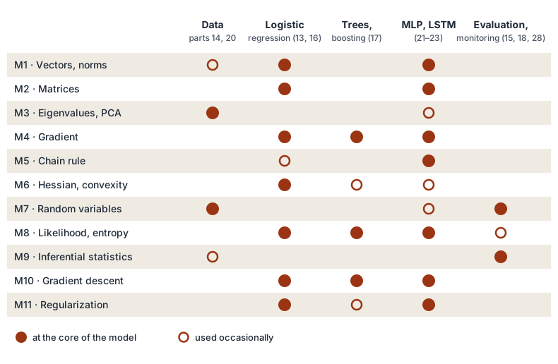
Map of maths concepts M1 to M11 and the models where they show up: data, logistic regression, trees and boosting, MLP and LSTM, evaluation and monitoring.

Three rows of the map deserve a word:

the gradient, gradient descent and cross-entropy are everywhere, trees included: gradient boosting is gradient descent over functions (M10), and LightGBM even takes a Newton step in each leaf (M6);
inferential statistics trains no model at all, but it’s what decides whether one model beats another, and whether production data has drifted (part 28);
random variables sit in the “Data” column: an autocorrelated sample can’t be split into train/test like an independent one (M7, part 14).

Code example

Logistic regression, entirely in NumPy

We reuse the memory-region generator from M9 to M11 and the 4 domain features. The model, its loss, its gradient, its Hessian and its two optimizers are written by hand. scikit-learn is used for only two things: getting the same train/test split as in the previous articles, and checking the result at the end.

import numpy as np
from sklearn.model_selection import train_test_split   # only to get the same test set as M9–M11


def make_regions(n, rng):
    """Synthetic memory regions (same generator as M9–M11): label 1 = hot in the next window."""
    rate = rng.gamma(0.6, 4, n)
    recent_accesses = rng.poisson(rate)
    since_last = np.round(rng.exponential(30 / (1 + recent_accesses)), 1)
    periodic = rng.binomial(1, 0.25, n)
    before_peak = rng.integers(0, 12, n)
    logit = (0.9 * np.log1p(recent_accesses) - 0.05 * since_last
             + 3.0 * periodic * (before_peak < 3) - 1.5 + rng.normal(0, 0.8, n))
    X = np.column_stack([recent_accesses, since_last, periodic, before_peak])
    return X, (logit > 0).astype(int)


def domain_features(X):
    return np.column_stack([np.log1p(X[:, 0]), X[:, 1], X[:, 2], X[:, 2] * (X[:, 3] < 3)])


def f1(y, yhat):
    tp = np.sum((yhat == 1) & (y == 1))
    return 2 * tp / (np.sum(yhat == 1) + np.sum(y == 1))


rng = np.random.default_rng(0)
X, y = make_regions(5000, rng)
Xtr, Xte, ytr, yte = train_test_split(X, y, test_size=0.3, random_state=0, stratify=y)
Ftr, Fte = domain_features(Xtr), domain_features(Xte)
mu, sd = Ftr.mean(axis=0), Ftr.std(axis=0)                     # M1: standardize with training stats
A_tr = np.column_stack([np.ones(len(Ftr)), (Ftr - mu) / sd])   # M2: one matrix, one row per region
A_te = np.column_stack([np.ones(len(Fte)), (Fte - mu) / sd])
lam = 1e-3                                                     # M11: L2 penalty (not on the intercept)
mask = np.r_[0.0, np.ones(4)]


def sigmoid(z):
    return 1 / (1 + np.exp(-z))


def loss(w, A, y):
    """M8: mean negative log-likelihood of a Bernoulli, + M11: (λ/2)‖w‖²."""
    p = sigmoid(A @ w)                                         # M1 + M2: dot products in bulk
    return -np.mean(y * np.log(p) + (1 - y) * np.log(1 - p)) + lam / 2 * np.sum(mask * w ** 2)


def gradient(w, A, y):
    """M4 + M5: chain rule, σ' = σ(1 − σ) cancels out, leaving Aᵀ(p − y)/n."""
    return A.T @ (sigmoid(A @ w) - y) / len(y) + lam * mask * w


def hessian(w, A):
    """M6: Aᵀ S A / n with S = diag(p(1 − p)): positive semi-definite, so the loss is convex."""
    p = sigmoid(A @ w)
    return (A * (p * (1 - p))[:, None]).T @ A / len(A) + lam * np.diag(mask)


# 1. check the gradient with finite differences (M4)
w = rng.normal(size=5)
h = 1e-6
num = np.array([(loss(w + h * e, A_tr, ytr) - loss(w - h * e, A_tr, ytr)) / (2 * h) for e in np.eye(5)])
print(f"analytic / numerical gradient gap: {np.abs(num - gradient(w, A_tr, ytr)).max():.1e}")

# 2. Newton (M6 + M10): w ← w − H⁻¹ ∇L
w = np.zeros(5)
for it in range(1, 8):
    w = w - np.linalg.solve(hessian(w, A_tr), gradient(w, A_tr, ytr))
    print(f"Newton iteration {it}: loss = {loss(w, A_tr, ytr):.6f} | ‖∇L‖ = {np.linalg.norm(gradient(w, A_tr, ytr)):.1e}")
ev = np.linalg.eigvalsh(hessian(w, A_tr))
print(f"Hessian at the optimum: eigenvalues from {ev[0]:.4f} to {ev[-1]:.4f} (all > 0), condition number {ev[-1] / ev[0]:.1f}")

# 3. gradient descent (M10) with step 1/λ_max, for comparison
w_gd, L_star, step = np.zeros(5), loss(w, A_tr, ytr), 1 / ev[-1]
for k in range(1, 5001):
    w_gd -= step * gradient(w_gd, A_tr, ytr)
    if loss(w_gd, A_tr, ytr) - L_star < 1e-6:
        break
print(f"GD (step = 1/λ_max = {step:.2f}): gap < 1e-6 after {k} iterations")

# 4. the model, read and evaluated
print("weights (intercept, log_accesses, since_last, periodic, peak_imminent):", w.round(3))
p_te = sigmoid(A_te @ w)
print(f"test F1 (threshold 0.5) = {f1(yte, (p_te > 0.5).astype(int)):.3f}")

# 5. check (the only "ready-made" ML line): scikit-learn, same penalty
from sklearn.linear_model import LogisticRegression
ref = LogisticRegression(C=1 / (lam * len(ytr)), tol=1e-10, max_iter=10_000).fit(A_tr[:, 1:], ytr)
print(f"max gap with scikit-learn: {np.abs(np.r_[ref.intercept_, ref.coef_[0]] - w).max():.1e}")

Step	What we observe	Concept
Gradient check	gap of $1.1 \times 10^{-10}$ with finite differences	M4, M5
Newton, iterations 4 → 7	$\lVert \nabla L \rVert$ : $2.9 \times 10^{-3}$ , $3.0 \times 10^{-4}$ , $3.7 \times 10^{-6}$ , $5.8 \times 10^{-10}$	M6, M10
Hessian at the optimum	eigenvalues from 0.0056 to 0.2000, all positive, condition number 35.8	M6
Gradient descent	146 iterations to get within $10^{-6}$ of the optimal loss (0.274160)	M10
Final check	gap of $5.1 \times 10^{-8}$ with scikit-learn’s weights

What we read:

Newton converges in 7 iterations, and quadratic convergence shows in the gradient column: over the last iterations, each norm is about 40 times the square of the previous one ( $2.9 \times 10^{-3}$ , then $3.0 \times 10^{-4}$ , $3.7 \times 10^{-6}$ , $5.8 \times 10^{-10}$ ). The number of correct digits doubles at each step. Gradient descent, with the classic step $1/\lambda_{\max} = 5$ , needs 146;
the condition number is 35.8 at the optimum, versus 3 at $w = 0$ in M10. The Hessian weights each region by $p_i(1 - p_i)$ : once the model is trained, most regions are predicted confidently and weigh little, and the curvature becomes more uneven. Newton doesn’t care, gradient descent pays for it;
the weights can be read (standardized features): since_last ( $-2.001$ ), log_accesses ( $+1.625$ ) and peak_imminent ( $+1.502$ ) carry the model, while periodic ( $+0.041$ ) is useless once the interaction is given. That’s what M11’s $L_1$ path had found;
test F1: 0.689, on par with M9’s LR with features (0.686, with a different scale and regularization) and with LightGBM (0.681).

The MLP, entirely in NumPy

This time the model gets the 4 raw features, standardized, without the log or the interaction. 16 hidden units, hand-written backpropagation, AdamW on mini-batches of 64.

# continues the previous block (make_regions, f1, sigmoid, Xtr, Xte, ytr, yte already defined)
# an MLP on the 4 RAW features (standardized): it has to find the "periodic × peak imminent" interaction on its own
m_r, s_r = Xtr.mean(axis=0), Xtr.std(axis=0)
Rtr, Rte = (Xtr - m_r) / s_r, (Xte - m_r) / s_r
H = 16                                                         # hidden units


def init(rng):
    """He initialization (M7: variance 2/fan_in) for ReLU layers."""
    return {"W1": rng.normal(0, np.sqrt(2 / 4), (4, H)), "b1": np.zeros(H),
            "W2": rng.normal(0, np.sqrt(2 / H), H), "b2": 0.0}


def forward(P, X):
    Z1 = X @ P["W1"] + P["b1"]                                 # M2: an affine transformation...
    A1 = np.maximum(Z1, 0)                                     # ... then a non-linearity
    return Z1, A1, sigmoid(A1 @ P["W2"] + P["b2"])


def backward(P, X, y):
    """M5: backpropagation written by hand, layer by layer."""
    Z1, A1, p = forward(P, X)
    n = len(y)
    d2 = (p - y) / n                                           # ∂L/∂z2, same simplification as LR
    d1 = np.outer(d2, P["W2"]) * (Z1 > 0)                      # ∂L/∂z1: back through W2, then ReLU's derivative
    return {"W1": X.T @ d1, "b1": d1.sum(axis=0), "W2": A1.T @ d2, "b2": d2.sum()}


def log_loss(P, X, y):
    p = np.clip(forward(P, X)[2], 1e-12, 1 - 1e-12)
    return -np.mean(y * np.log(p) + (1 - y) * np.log(1 - p))


# 1. check backpropagation with finite differences (M4) on 200 examples
P = init(np.random.default_rng(1))
Xs, ys = Rtr[:200], ytr[:200]
g = backward(P, Xs, ys)
gap = 0.0
for k, idx in (("W1", (0, 0)), ("W1", (3, 7)), ("W2", (5,)), ("b1", (2,))):
    plus, minus = {c: np.copy(a) for c, a in P.items()}, {c: np.copy(a) for c, a in P.items()}
    plus[k][idx] += 1e-6
    minus[k][idx] -= 1e-6
    num = (log_loss(plus, Xs, ys) - log_loss(minus, Xs, ys)) / 2e-6
    gap = max(gap, abs(num - g[k][idx]))
print(f"backpropagation / finite differences gap: {gap:.1e}")

# 2. train with AdamW (M10 + M11), mini-batches of 64
P, rng_b = init(np.random.default_rng(1)), np.random.default_rng(2)
m = {k: np.zeros_like(v) for k, v in P.items()}
v = {k: np.zeros_like(v) for k, v in P.items()}
eta, wd, t = 0.01, 1e-4, 0
for epoch in range(1, 101):
    order = rng_b.permutation(len(ytr))
    for start in range(0, len(ytr), 64):
        i = order[start:start + 64]
        g, t = backward(P, Rtr[i], ytr[i]), t + 1
        for k in P:
            m[k] = 0.9 * m[k] + 0.1 * g[k]
            v[k] = 0.999 * v[k] + 0.001 * g[k] ** 2
            P[k] = P[k] - eta * (m[k] / (1 - 0.9 ** t)) / (np.sqrt(v[k] / (1 - 0.999 ** t)) + 1e-8)
            if k.startswith("W"):
                P[k] = P[k] * (1 - eta * wd)                   # AdamW: weight decay applied separately
    if epoch in (1, 10, 50, 100):
        p_te_mlp = forward(P, Rte)[2]
        print(f"epoch {epoch:>3}: train log-loss = {log_loss(P, Rtr, ytr):.4f} | test = {log_loss(P, Rte, yte):.4f} "
              f"| test F1 = {f1(yte, (p_te_mlp > 0.5).astype(int)):.3f}")

# 3. did the MLP find the interaction? mean predicted probability per group (test set)
per, peak = Xte[:, 2] == 1, Xte[:, 3] < 3
for name, grp in (("periodic, peak imminent", per & peak), ("periodic, peak far away", per & ~peak),
                  ("not periodic", ~per)):
    print(f"{name:<24}: mean MLP p = {p_te_mlp[grp].mean():.3f} | actual rate = {yte[grp].mean():.3f} | n = {grp.sum()}")

Epoch	Training log-loss	Test log-loss	Test F1
1	0.3308	0.3496	0.643
10	0.2864	0.2980	0.684
50	0.2780	0.3004	0.692
100	0.2750	0.3011	0.682

Group (test set)	Mean $p$ predicted by the MLP	Actual rate	Regions
periodic, peak imminent	0.751	0.811	106
periodic, peak far away	0.197	0.170	288
not periodic	0.205	0.177	1,106

What we read:

backpropagation is correct: a gap of $8.8 \times 10^{-11}$ with finite differences. That’s the test to run every time you write a gradient by hand;
the MLP found the interaction on its own: it gives 0.751 to periodic regions whose peak is coming up, and 0.197 to the other periodic regions, just like the non-periodic ones. LR on these same raw features couldn’t make that distinction (F1 of 0.582 in M9); the MLP reaches 0.682, on par with the LR that was handed the right features;
overfitting shows: the training log-loss keeps falling until the end (0.2750), while the test log-loss bottoms out around epoch 10 (0.2980) and then rises. The F1 fluctuates between 0.682 and 0.692 with no clear trend. You’d stop training earlier, on a validation set (early stopping, part 22).

Compare and look inside: M9 and M3

# continues the two previous blocks
from scipy import stats

# 1. M9: paired bootstrap and McNemar, LR + features (NumPy) versus MLP on raw features
pred_lr, pred_mlp = (p_te > 0.5).astype(int), (p_te_mlp > 0.5).astype(int)
idx = np.random.default_rng(0).integers(0, len(yte), (2000, len(yte)))
delta = np.array([f1(yte[i], pred_mlp[i]) - f1(yte[i], pred_lr[i]) for i in idx])
lo, hi = np.percentile(delta, [2.5, 97.5])
ok_lr, ok_mlp = pred_lr == yte, pred_mlp == yte
n01, n10 = int(np.sum(ok_lr & ~ok_mlp)), int(np.sum(~ok_lr & ok_mlp))
print(f"ΔF1 (MLP − LR) = {f1(yte, pred_mlp) - f1(yte, pred_lr):+.3f}, 95% CI [{lo:+.3f}, {hi:+.3f}] "
      f"| McNemar: {n01} vs {n10}, p = {stats.binomtest(n01, n01 + n10, 0.5).pvalue:.2g}")

# 2. M3: PCA of the hidden layer. How many dimensions does the MLP really use?
A1 = forward(P, Rte)[1]
dead = int(np.sum(A1.max(axis=0) == 0))
s = np.linalg.svd(A1 - A1.mean(axis=0), compute_uv=False)
share = np.cumsum(s ** 2) / np.sum(s ** 2)
print(f"never-active units: {dead} of {H} | variance explained by 1, 2, 3, 4 components: {share[:4].round(3)}")

M9: the two models are tied. The MLP scores $-0.007$ in F1 against the LR with features, with a paired interval $[-0.024, +0.012]$ that contains 0. On the 39 regions where they disagree, LR is right 24 times and the MLP 15 times, $p = 0.2$ : nothing significant. The right conclusion isn’t “LR is better”, it’s “the MLP recovers, unaided, what feature engineering had contributed”. On real traces, where nobody knows the right interaction in advance, that’s the whole point.
M3: the hidden layer lives in few dimensions. None of the 16 units is dead (all of them fire on at least one test region). But the PCA of their activations shows that 4 directions carry 88.1% of the variance (40.5% for the first, 65.7% for two, 79.6% for three). The input has 4 dimensions, the network spreads it over 16 coordinates, and most of it stays in a low-dimensional subspace, like M3’s point cloud.

Hands-on exercise

By hand. Derive the gradient and the Hessian of the regularized log-loss starting from $\sigma'(z) = \sigma(z)(1 - \sigma(z))$ . Show that the Hessian is positive definite as soon as $\lambda > 0$ and the intercept column isn’t zero.
Newton versus gradient. Redo the first block with $\lambda = 0$ , then $\lambda = 0.1$ . How do the number of Newton iterations, the number of gradient descent iterations and the Hessian’s condition number at the optimum change? Relate the answer to the $\lambda I$ term.
Two hidden layers. Add a second hidden layer of 8 units to the MLP. Rewrite backward (one more $\delta$ ) and check it with finite differences before training: the gap should stay under $10^{-6}$ .
Early stopping. Hold out 20% of the training set for validation. Train the MLP for 100 epochs, keeping the parameters with the best validation log-loss. At which epoch does it stop? Compare the test F1 with the epoch-100 one, then run McNemar’s test between the two.
The running project, rewritten with the maths. Take part 24’s project and annotate each step with the concept that justifies it: standardization (M1), a time-based rather than random split (M7), the loss (M8), the optimizer and its learning rate (M10), regularization (M11), comparing models (M9), monitoring drift (M9), the LSTM’s backpropagation through time (M5). If a step has no justification, that’s a signal.
Bonus. Give the MLP the 4 domain features instead of the raw ones. Does it gain anything over LR? What does the paired bootstrap say?

Hint for question 1: for any $v \ne 0$ , $v^\top \nabla^2 L\, v = \frac{1}{n}\sum_i p_i(1 - p_i)(x_i^\top v)^2 + \lambda \|v_{\text{no intercept}}\|^2$ . The second term is strictly positive as soon as $v$ has a non-intercept component; otherwise $x_i^\top v = v_0 \ne 0$ for every $i$ , and the first one is.

Review of the maths programme, and what comes next

What was covered. Three blocks, each answering one question:

how to represent: vectors, norms, matrices, eigenvalues and SVD (M1 to M3);
how to learn: the gradient, the chain rule, the Hessian, gradient descent and regularization (M4 to M6, M10, M11);
how to reason under uncertainty: random variables, likelihood, entropy and inferential statistics (M7 to M9).

With that, you can read a fit() as a sequence of equations, which was the goal of the roadmap.

What’s left to deepen, when the need arises:

time series: autocorrelation, stationarity, block validation. DAMON traces are time series, and it’s the topic we skimmed the most (M7, M9);
numerical linear algebra: stability, float32 versus float64, why you solve a system instead of inverting a matrix;
convex optimization beyond KKT: duality, proximal methods, convergence guarantees for SGD;
Bayesian inference beyond the Gaussian prior: uncertainty on predictions, useful to decide when a prediction is confident enough to move a page to zswap.

What’s next. The technical phase starts at part 13 and takes all of this up with real tools: leakage-free data preparation, evaluation, linear models, trees, PyTorch, LSTMs, then production. The running project (part 24) will finally replace the synthetic regions with real DAMON traces, and that’s where the thesis begins for real.

Further resources

Deisenroth, Faisal and Ong, Mathematics for Machine Learning, part II (chapters 8 to 12): regression, PCA, Gaussian mixtures and SVMs derived with the tools of part I, free online.
Goodfellow, Bengio and Courville, Deep Learning, part I (chapters 2 to 5): the complete maths review for deep learning, free online.
Bishop, Pattern Recognition and Machine Learning, section 4.3 (logistic regression and IRLS) and chapter 5 (neural networks and backpropagation).
Andrew Ng, Stanford CS229 lecture notes, the part on logistic regression and Newton’s method.
Michael Nielsen, Neural Networks and Deep Learning, chapter 2: backpropagation derived step by step, free online.
Andrej Karpathy, micrograd: an autodiff engine in about a hundred lines, to watch M5’s chain rule become a tool.

What you should be able to do before moving on

Derive the loss, gradient and Hessian of logistic regression, and say where each term comes from (M1, M2, M4 to M8)
Explain why logistic regression is convex and an MLP isn’t
Implement logistic regression with no library, with gradient descent and with Newton
Write the backpropagation of a one-hidden-layer MLP and check it with finite differences
Explain each step of training mathematically: initialization, loss, gradient, step, regularization, stopping
Compare two models with a paired bootstrap and McNemar, and correctly conclude to a tie
Place each concept from M1 to M11 in at least one model of the technical phase

Next part: Part 13 · The supervised ML framework, revisited. The start of the technical phase: we take supervised ML back up with the maths in hand.