M2 · Matrices as transformations

Mastering AI · Required Maths · Week 1 (linear algebra) · Part 2

Goal of this step

In M1 we handled vectors one at a time. In ML we process them in batches, and the tool for that is the matrix. But a matrix isn’t just a table of numbers: it’s a transformation of space. That reading makes it obvious what a network layer does, why activations are essential, and where the linear regression formula comes from.

By the end of this article you’ll be able to:

• read a matrix as a transformation, column by column;
• interpret the matrix product as composition;
• tie rank, determinant and invertibility to a geometric picture;
• derive and solve least squares;
• show why stacking linear layers without activations is pointless.

---

Key concepts

1. One matrix, two readings

Intuition. An $m \times n$ matrix $A$ takes a vector in $\mathbb{R}^n$ and returns one in $\mathbb{R}^m$ . It is linear: it respects sums and scalar multiplication, $A(\alpha u + \beta v) = \alpha Au + \beta Av$ . Lines stay lines, the origin stays put, and a regular grid stays a regular grid, possibly skewed.

The product $Ax$ can be read two ways, and you need both.

Row reading: dot products. Each output component is the dot product of a row of $A$ with $x$ (M1):

$$(Ax)_i = \sum_{j} A_{ij}\, x_j = \langle a_i, x \rangle$$

This is the “neurons” reading: each row is a neuron measuring how aligned $x$ is with its direction.

Column reading: a combination. $Ax$ is a combination of the columns of $A$ , weighted by the coordinates of $x$ :

$$Ax = x_1\, A_{:,1} + x_2\, A_{:,2} + \dots + x_n\, A_{:,n}$$

Key consequence: the columns of $A$ are the images of the basis vectors. To know what a $2 \times 2$ matrix does, just look at where it sends $e_1 = (1, 0)$ and $e_2 = (0, 1)$ . Everything else follows by linearity.

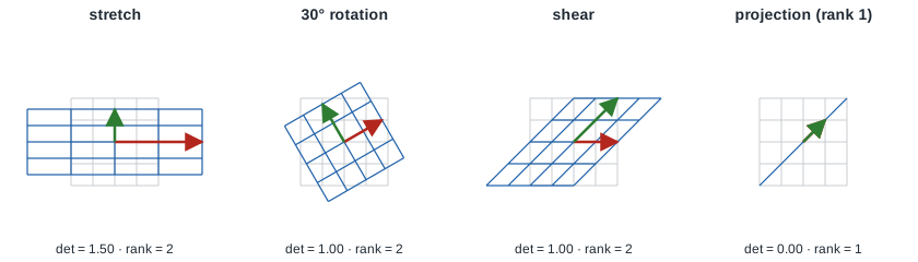
In each panel, the gray grid is the input space and the blue one its image. The red arrow is the matrix’s first column (the image of $e_1$ ), the green arrow the second (the image of $e_2$ ). The last panel shows a matrix squashing the whole plane onto a line: we’ll come back to it with rank.

2. Matrix product = composition

Intuition. Applying $B$ , then $A$ , is applying a single transformation, written $AB$ . Read right to left, like $f(g(x))$ .

$$A(Bx) = (AB)\,x$$

Two consequences:

• sizes must chain: $(m \times k)(k \times n) \to (m \times n)$ ;
• order matters: in general $AB \neq BA$ . Rotating then stretching isn’t the same as stretching then rotating.

3. Data as a matrix

Your dataset is an $n \times d$ matrix $X$ : one row per example, one column per feature. For a linear model with weights $w \in \mathbb{R}^d$ , all predictions come out at once:

$$\hat y = Xw \in \mathbb{R}^n$$

That’s the row reading: each prediction is the dot product of an example with $w$ . It’s also why NumPy and GPUs are fast: one matrix multiplication replaces a loop over examples.

4. Rank, determinant, inverse

Intuition. Some transformations “squash” space into a lower dimension. Once squashed, there’s no going back.

• Rank: the dimension of the output space actually reached. A rank-1 $2 \times 2$ matrix squashes the plane onto a line.
• Null space: vectors sent to $0$ . If it contains anything besides $0$ , two different inputs give the same output, and information is lost.
• Determinant (square matrices): the area (or volume) scaling factor. $\det A = 2$ doubles areas; $\det A = 0$ squashes everything into a lower dimension; a negative determinant flips orientation.
• Inverse: $A^{-1}$ undoes $A$ , i.e. $A^{-1}A = I$ . It exists if and only if $\det A \neq 0$ , i.e. $A$ has full rank.

On the ML side: if two features are perfectly correlated (say the same measurement in ms and in s), the columns of $X$ are dependent, $X^\top X$ isn’t invertible, and linear regression has no unique solution. That’s multicollinearity, one of the reasons regularization exists (M11, part 16).

5. Least squares

Intuition. We look for $w$ such that $Xw$ is as close as possible to $y$ . But $Xw$ is necessarily a combination of the columns of $X$ (column reading). So we’re looking for the point in that column space closest to $y$ : the projection of $y$ onto it (M1).

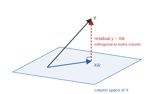
At the optimum, the residual $y - Xw$ is orthogonal to every column of $X$ :

$$\begin{aligned} X^\top (y - Xw) = 0 \quad&\Longrightarrow\quad X^\top X\, w = X^\top y \\ &\Longrightarrow\quad \hat w = (X^\top X)^{-1} X^\top y \end{aligned}$$

These are the normal equations. We’ll find them again with calculus (setting the MSE gradient to zero, M4), but the geometric argument is more telling.

In practice you never invert $X^\top X$ explicitly: it’s slow and numerically unstable. You solve the system (np.linalg.solve), or better, go through a decomposition such as the SVD (np.linalg.lstsq, M3).

6. A network layer = a matrix (+ a non-linearity)

A dense layer from $d$ inputs to $h$ neurons computes:

$$h = \sigma(Wx + b), \qquad W \in \mathbb{R}^{h \times d}$$

Without the activation $\sigma$ , two successive layers give:

$$W_2 (W_1 x) = (W_2 W_1)\, x$$

i.e. a single matrix. Stacking 10 linear layers is still a linear model. The non-linearity (ReLU, sigmoid…) is what gives the network its capacity to represent complex functions (part 21).

---

Code example

Watching a matrix transform the plane

This script reproduces the figure from section 1: a grid (gray) and its image under four matrices (blue). The red and green arrows are the images of $e_1$ and $e_2$ , i.e. the matrix’s columns.

import numpy as np
import matplotlib.pyplot as plt

matrices = {
    "stretch": np.array([[2.0, 0.0], [0.0, 0.75]]),
    "rotation 30°": np.array([[np.cos(np.pi / 6), -np.sin(np.pi / 6)],
                              [np.sin(np.pi / 6),  np.cos(np.pi / 6)]]),
    "shear": np.array([[1.0, 1.0], [0.0, 1.0]]),
    "projection (rank 1)": np.array([[1.0, 1.0], [1.0, 1.0]]) / 2,
}

lines = np.linspace(-1, 1, 9)
fig, axes = plt.subplots(1, 4, figsize=(16, 4))
for ax, (name, A) in zip(axes, matrices.items()):
    for c in lines:
        for seg in (np.stack([np.full(50, c), np.linspace(-1, 1, 50)]),
                    np.stack([np.linspace(-1, 1, 50), np.full(50, c)])):
            ax.plot(*seg, c="lightgray", lw=0.6)
            ax.plot(*(A @ seg), c="tab:blue", lw=0.8)
    e1, e2 = A[:, 0], A[:, 1]   # images of the basis vectors = columns
    ax.arrow(0, 0, *e1, color="tab:red", width=0.02, length_includes_head=True)
    ax.arrow(0, 0, *e2, color="tab:green", width=0.02, length_includes_head=True)
    ax.set_title(f"{name}\ndet = {np.linalg.det(A):.2f}, rank = {np.linalg.matrix_rank(A)}")
    ax.set_aspect("equal")
    ax.set_xlim(-2.5, 2.5)
    ax.set_ylim(-2, 2)
plt.tight_layout()
plt.show()

Matrix	det	rank	What happens
stretch	1.50	2	areas multiplied by 1.5
rotation 30°	1.00	2	everything turns, nothing changes size
shear	1.00	2	the square becomes a parallelogram of equal area
projection	0.00	1	the whole plane is squashed onto the diagonal: no way back

The shear is instructive: the shape changes completely, but the area is preserved, and the determinant says so.

Order matters

import numpy as np

R = np.array([[np.cos(np.pi / 6), -np.sin(np.pi / 6)],
              [np.sin(np.pi / 6),  np.cos(np.pi / 6)]])   # 30° rotation
S = np.array([[2.0, 0.0], [0.0, 0.75]])                    # stretch
x = np.array([1.0, 1.0])

print("R(Sx) =", R @ (S @ x), "| (RS)x =", (R @ S) @ x)   # identical: composition
print("RS == SR ?", np.allclose(R @ S, S @ R))            # False: order matters

Least squares, three ways

import numpy as np
from sklearn.linear_model import LinearRegression

rng = np.random.default_rng(0)
n, d = 200, 3
X = rng.normal(size=(n, d))
w_true = np.array([2.0, -1.0, 0.5])
y = X @ w_true + rng.normal(0, 0.3, n)

w_normal = np.linalg.solve(X.T @ X, X.T @ y)            # normal equations
w_lstsq, *_ = np.linalg.lstsq(X, y, rcond=None)         # stable solver (SVD)
w_sklearn = LinearRegression(fit_intercept=False).fit(X, y).coef_

print("w normal  :", w_normal.round(4))
print("w lstsq   :", w_lstsq.round(4))
print("w sklearn :", w_sklearn.round(4))

residual = y - X @ w_lstsq
print("X^T (y - Xw) =", (X.T @ residual).round(10), "(residual orthogonal to the columns)")

All three methods give $\hat w = (1.9737,\ -1.0293,\ 0.5165)$ , close to the true weights $(2, -1, 0.5)$ ; the gap comes from the noise. The last line prints a zero vector: the residual is indeed orthogonal to every column of $X$ , exactly as the geometric argument predicts.

Two linear layers = one

A mini-network: 9 features (those from part 14), 16 hidden neurons, 1 output, on 1,000 examples.

import numpy as np

rng = np.random.default_rng(0)
W1 = rng.normal(size=(16, 9))     # 9 features -> 16 neurons
W2 = rng.normal(size=(1, 16))     # 16 neurons -> 1 output
X = rng.normal(size=(9, 1000))    # 1000 examples, as columns

no_activation = W2 @ (W1 @ X)
one_layer = (W2 @ W1) @ X
print("Two linear layers == one layer W2W1 ?", np.allclose(no_activation, one_layer))

relu = lambda z: np.maximum(z, 0)
with_relu = W2 @ relu(W1 @ X)
print("With ReLU == one layer W2W1 ?", np.allclose(with_relu, one_layer))

Without activation, the two-layer network is exactly a $1 \times 9$ matrix: we paid for 160 parameters to get a model worth 9. With a ReLU in between, the equality breaks: the network is no longer linear.

---

Hands-on exercise

1. Build a matrix from what it does. Write the matrix sending $e_1$ to $(0, 1)$ and $e_2$ to $(-1, 0)$ . Which transformation is it? Compute its determinant and check by plotting the grid.
2. Squashing space. For $A = \begin{pmatrix} 1 & 2 \\ 2 & 4 \end{pmatrix}$ , compute rank and determinant. Find a non-zero $v$ with $Av = 0$ . What happens with np.linalg.inv(A)?
3. Multicollinearity. In the least squares code, add a 4th column equal to 2 * X[:, 0]. What happens to the rank of $X$ , the condition number of $X^\top X$ (np.linalg.cond), and the coefficients returned by solve and by lstsq? Which solver survives?
4. Compute cost. Time X @ w with time.perf_counter for $X$ of size $10^6 \times 9$ , then a Python loop doing the $10^6$ dot products one by one. What’s the ratio? Relate it to the inference budget of a daemon scoring thousands of memory regions every 100 ms.
5. Running project. For a logistic regression on the 9 features of part 14, write the shapes of $X$ , $w$ and $Xw$ when scoring 4,096 regions at once. How many multiplications is that?

Hint for question 2: the second column is twice the first, so the columns only span a line.

---

Further resources

• 3Blue1Brown, Essence of Linear Algebra, episodes 3–7 (linear transformations, multiplication, determinant, inverse and rank): this article’s geometric intuition, animated.
• Gilbert Strang, MIT 18.06 Linear Algebra, lectures 1–3 and 15–16 (projections and least squares), free on video.
• Deisenroth et al., Mathematics for Machine Learning, chapter 2 (linear algebra) and section 9.2 (least squares).
• On this blog: Linear regression, low-level.

---

What you should be able to do before moving on

• Read a product $Ax$ by rows (dot products) and by columns (combination)
• Build a transformation’s matrix from the images of $e_1$ and $e_2$
• Explain why $AB \neq BA$ in general
• Interpret rank, null space and determinant geometrically, and know when a matrix is invertible
• Derive the normal equations from the orthogonality of the residual
• Explain why a network without activations is a linear model

Next part: M3 · Eigenvalues, SVD and PCA. We look for the directions a matrix only stretches, and derive PCA and a stable way to solve least squares.