M4 · Derivatives, partial derivatives and the gradient

Mastering AI · Required Maths · Week 2 (calculus) · Part 4

Goal of this step

Training a model means looking for the parameters that minimize the loss. To know which way to move the parameters, we need one thing: the gradient. This calculus week starts with it.

By the end of this article you’ll be able to:

• read a derivative as a local slope and compute it numerically;
• compute partial derivatives and assemble a gradient;
• explain why the gradient points in the direction of steepest ascent;
• derive by hand the gradient of the MSE and the log-loss, and check it numerically.

---

Key concepts

1. The derivative: a local slope

Intuition. Zoom in far enough on a smooth curve and it starts looking like a straight line. The slope of that line is the derivative. It says: “if I nudge $x$ a tiny bit, how much does $f$ move?”.

It is the limit of the slopes of secant lines:

$$f'(x) = \lim_{h \to 0} \frac{f(x+h) - f(x)}{h}$$

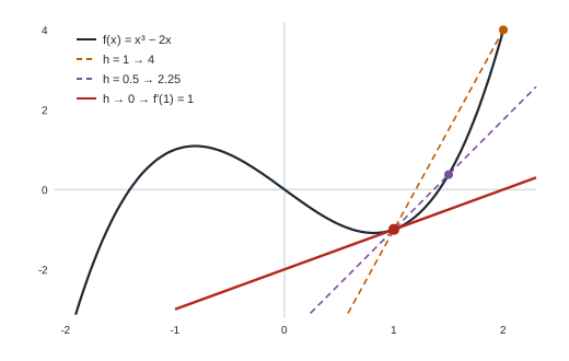
In the figure, the secant between $x = 1$ and $x = 2$ has slope 4, the one between $1$ and $1.5$ slope 2.25. As $h$ goes to 0, we get the tangent with slope $f'(1) = 3 \cdot 1^2 - 2 = 1$ .

Rules you use all the time:

Function	Derivative
$x^k$	$k\,x^{k-1}$
$e^x$	$e^x$
$\ln x$	$1/x$
$u + v$	$u' + v'$
$u \cdot v$	$u'v + uv'$
$u(v(x))$	$u'(v(x))\cdot v'(x)$ (chain rule, see M5)

Numerically, we approximate the derivative with finite differences. The centered version is far more accurate than the forward one:

$$f'(x) \approx \frac{f(x+h) - f(x-h)}{2h}$$

The forward version’s error is proportional to $h$ , the centered one’s to $h^2$ (we’ll prove it with Taylor in M6). But beware: if $h$ is too small, floating-point rounding errors take over.

2. Partial derivatives and the gradient

Intuition. A loss depends on many parameters $w_1, \dots, w_d$ . The partial derivative $\partial f / \partial w_i$ measures the effect of a small change in $w_i$ alone, all others frozen. The gradient stacks all partial derivatives into a vector:

$$\nabla f(w) = \left(\frac{\partial f}{\partial w_1}, \dots, \frac{\partial f}{\partial w_d}\right)$$

Example: for $g(w) = \frac{w_1^2}{4} + w_2^2$ , we get $\nabla g(w) = \left(\frac{w_1}{2},\ 2w_2\right)$ , so $\nabla g(2, 1) = (1, 2)$ .

3. Why the gradient points uphill fastest

Intuition. Standing on a hill, which way climbs fastest? The gradient answers.

Taking a small step $\varepsilon u$ in a unit direction $u$ changes the function by about:

$$f(w + \varepsilon u) - f(w) \approx \varepsilon\, \langle \nabla f(w), u \rangle$$

That’s a dot product (M1): it’s largest when $u$ is aligned with $\nabla f$ , where it equals $\|\nabla f\|$ . It’s zero when $u$ is perpendicular to the gradient: you stay at the same height. Three consequences:

• $\nabla f$ gives the direction of steepest ascent, and $\|\nabla f\|$ the slope in that direction;
• $-\nabla f$ gives the direction of steepest descent: the whole idea of gradient descent (M10);
• the gradient is perpendicular to level sets (the curves where $f$ is constant).

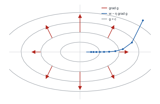
In the figure, the ellipses are level sets of $g$ . The red arrows (the gradient) cross each ellipse at a right angle. The blue path applies the rule $w \leftarrow w - \eta \nabla g(w)$ : it heads to the minimum, quickly in the vertical direction (where $g$ is steeper), then more slowly horizontally.

4. The gradients of the losses we use

MSE of linear regression. With $L(w) = \frac{1}{n}\|Xw - y\|^2$ :

$$\nabla L(w) = \frac{2}{n} X^\top (Xw - y)$$

Setting it to zero gives $X^\top X w = X^\top y$ : exactly the normal equations we found geometrically in M2.

Log-loss of logistic regression. With $p_i = \sigma(x_i^\top w)$ and $\sigma(z) = \frac{1}{1 + e^{-z}}$ , we use a remarkable property of the sigmoid:

$$\sigma'(z) = \sigma(z)\,\big(1 - \sigma(z)\big)$$

Differentiating $L(w) = -\frac{1}{n}\sum_i \big[y_i \log p_i + (1 - y_i)\log(1 - p_i)\big]$ , almost everything cancels:

$$\nabla L(w) = \frac{1}{n} X^\top \big(\sigma(Xw) - y\big)$$

The gradient is just the sum of the examples, weighted by the prediction error $p_i - y_i$ . With $L_2$ regularization $\frac{\lambda}{2}\|w\|^2$ , add $\lambda w$ . That’s the formula the logistic regression of part 16 uses.

---

Code example

Finite differences: forward vs centered

import numpy as np

def f(x):
    return x**3 - 2 * x

def f_prime(x):
    return 3 * x**2 - 2

x0 = 1.0
print("exact derivative:", f_prime(x0))
for h in (1e-1, 1e-3, 1e-5, 1e-8, 1e-12):
    forward = (f(x0 + h) - f(x0)) / h
    centered = (f(x0 + h) - f(x0 - h)) / (2 * h)
    print(f"h={h:.0e}  forward: error={abs(forward - f_prime(x0)):.2e}   centered: error={abs(centered - f_prime(x0)):.2e}")

$h$	Forward error	Centered error
$10^{-1}$	$3.1 \times 10^{-1}$	$1.0 \times 10^{-2}$
$10^{-3}$	$3.0 \times 10^{-3}$	$1.0 \times 10^{-6}$
$10^{-5}$	$3.0 \times 10^{-5}$	$9.5 \times 10^{-11}$
$10^{-8}$	$1.6 \times 10^{-8}$	$6.1 \times 10^{-9}$
$10^{-12}$	$8.9 \times 10^{-5}$	$8.9 \times 10^{-5}$

The forward version gains a factor of 100 when $h$ is divided by 100 (error in $h$ ). The centered one gains a factor of 10,000 (error in $h^2$ ). Below $h \approx 10^{-5}$ , rounding errors take over again: at $h = 10^{-12}$ , both are poor.

Numerical gradient and direction of steepest slope

import numpy as np

def g(w):
    return w[0] ** 2 / 4 + w[1] ** 2

def grad_g(w):
    return np.array([w[0] / 2, 2 * w[1]])

def numerical_grad(F, w, h=1e-5):
    gr = np.zeros_like(w)
    for i in range(len(w)):
        e = np.zeros_like(w)
        e[i] = h
        gr[i] = (F(w + e) - F(w - e)) / (2 * h)
    return gr

w = np.array([2.0, 1.0])
print("exact gradient    :", grad_g(w))
print("numerical gradient:", numerical_grad(g, w).round(6))

# try 360 unit directions: which one makes g increase fastest?
angles = np.linspace(0, 2 * np.pi, 360, endpoint=False)
dirs = np.stack([np.cos(angles), np.sin(angles)], axis=1)
slopes = dirs @ grad_g(w)
best = dirs[np.argmax(slopes)]
print("steepest direction:", best.round(3),
      "| normalized gradient:", (grad_g(w) / np.linalg.norm(grad_g(w))).round(3),
      "| max slope:", slopes.max().round(3), "= ||grad||:", np.linalg.norm(grad_g(w)).round(3))

The numerical gradient is exactly $(1, 2)$ . Among 360 directions, the best is $(0.454,\ 0.891)$ , less than a degree from the normalized gradient $(0.447,\ 0.894)$ , and the maximum slope is $2.236 = \|\nabla g\| = \sqrt 5$ .

Log-loss gradient: analytic vs numerical

We check the formula $\frac{1}{n}X^\top(\sigma(Xw) - y) + \lambda w$ on simulated data, then follow $-\nabla L$ and watch the loss fall.

import numpy as np

rng = np.random.default_rng(0)
n, d = 500, 3
X = rng.normal(size=(n, d))
w_true = np.array([1.5, -2.0, 0.5])

def sigmoid(z):
    return 1 / (1 + np.exp(-z))

y = (rng.random(n) < sigmoid(X @ w_true)).astype(float)

def log_loss(w, lam=0.0):
    p = sigmoid(X @ w)
    eps = 1e-12
    return -np.mean(y * np.log(p + eps) + (1 - y) * np.log(1 - p + eps)) + lam / 2 * w @ w

def grad_log_loss(w, lam=0.0):
    return X.T @ (sigmoid(X @ w) - y) / n + lam * w

def numerical_grad(F, w, h=1e-5):
    gr = np.zeros_like(w)
    for i in range(len(w)):
        e = np.zeros_like(w)
        e[i] = h
        gr[i] = (F(w + e) - F(w - e)) / (2 * h)
    return gr

w_test = rng.normal(size=d)
for lam in (0.0, 0.1):
    ga = grad_log_loss(w_test, lam)
    gn = numerical_grad(lambda v: log_loss(v, lam), w_test)
    print(f"lambda={lam}: max analytic/numerical gap = {np.abs(ga - gn).max():.1e}")

# follow -gradient: the loss goes down
w_k = np.zeros(d)
for k in range(201):
    if k in (0, 1, 5, 20, 50, 200):
        print(f"iteration {k:>3}: log-loss = {log_loss(w_k):.4f}, w = {w_k.round(3)}")
    w_k = w_k - 1.0 * grad_log_loss(w_k)

The gap between analytic and numerical gradients is around $10^{-11}$ : the formula is right. Descent takes the log-loss from $0.693$ ( $\ln 2$ , the loss of a model that always says 50%) to $0.463$ in 200 iterations, with $w \approx (1.19,\ -1.68,\ 0.24)$ . The signs and proportions of $w_{\text{true}} = (1.5,\ -2,\ 0.5)$ are recovered; the remaining gap comes from sampling noise on 500 examples.

This finite-difference check (the gradient check) is a habit to keep: whenever you write a gradient by hand, compare it with its numerical version.

---

Hands-on exercise

1. By hand. Compute $f'(x)$ for $f(x) = x^2 e^{-x}$ and $f(x) = \ln(1 + e^x)$ (the softplus function). Check with the centered difference. What do you notice about softplus’s derivative?
2. The MSE gradient. Write grad_mse(w) $= \frac{2}{n}X^\top(Xw - y)$ for a linear regression, check it with numerical_grad, then solve $\nabla L = 0$ with np.linalg.solve and compare with M2’s solution.
3. Level sets. For $h(w) = w_1^2 + w_1 w_2 + 2 w_2^2$ , compute $\nabla h$ . Plot a few level sets with plt.contour and overlay gradient arrows with plt.quiver. Check the orthogonality visually.
4. The step-size trap. In gradient descent on the log-loss, try a step of 10 then 50 instead of 1. What happens? (We’ll explain it in M6 and M10 with curvature.)
5. Running project. For a logistic model on the 9 features of part 14, what is the gradient’s dimension? How many operations does computing it cost for $n$ examples? Compare with the cost of a prediction.

Hint for question 1: softplus’s derivative is a function you already know very well.

---

Further resources

• 3Blue1Brown, Essence of Calculus, episodes 1–4: the derivative as a slope, animated.
• Khan Academy, Multivariable calculus, chapter Gradient and directional derivatives.
• Deisenroth et al., Mathematics for Machine Learning, chapter 5 (vector calculus), sections 5.1–5.3.
• CS231n (Stanford), notes on gradient checking.

---

What you should be able to do before moving on

• Explain a derivative as a local slope, with a drawing
• Compute a derivative numerically and pick a sensible $h$
• Compute a gradient by hand for a multivariable function
• Explain with the dot product why following $-\nabla f$ lowers $f$
• Derive $\frac{1}{n}X^\top(\sigma(Xw) - y)$ as the gradient of the log-loss
• Run a gradient check systematically

Next part: M5 · The chain rule and backpropagation. Differentiating a composition of functions is exactly what a neural network does during training.