M11 · Constraints and regularization, geometrically

Mastering AI · Required Maths · Week 4 (optimization) · Part 11

Goal of this step

In M10, gradient descent was free to go anywhere. In practice we often hold it back: we want small weights, or few of them. This article shows that regularizing means optimizing under a constraint, and that the shape of the constraint decides everything. It’s the proof promised since M1: why the corners of the $L_1$ diamond set weights exactly to zero.

By the end of this article you’ll be able to:

• solve a constrained optimization problem with a Lagrange multiplier, and interpret that multiplier as the price of the constraint;
• write the KKT conditions for an inequality constraint and recognize an active constraint;
• explain why penalizing by $\lambda\|\theta\|$ is the same as imposing $\|\theta\| \le t$ ;
• explain geometrically, then with calculus, why $L_1$ zeroes weights and $L_2$ shrinks them;
• read a regularization path and use it to select features on the running project;
• place SVMs and AdamW in this framework.

---

Key concepts

1. Constrained optimization: Lagrange multipliers

Intuition. You’re walking on a hill, but you must stay on a trail. The lowest point of the trail isn’t the bottom of the valley: it’s the spot where the trail grazes a level set without crossing it. There, the level set and the trail are tangent, so their normals are aligned. And the normal to a level set is the gradient (M4).

To minimize $f(\theta)$ subject to $g(\theta) = c$ , the condition reads:

$$\nabla f(\theta^*) + \lambda\, \nabla g(\theta^*) = 0, \qquad g(\theta^*) = c$$

The number $\lambda$ is the Lagrange multiplier. You get both equations by setting to zero the gradient of the Lagrangian:

$$\mathcal{L}(\theta, \lambda) = f(\theta) + \lambda\,\big(g(\theta) - c\big)$$

with respect to $\theta$ and $\lambda$ : the constraint is no longer an obstacle, just one more variable.

The price of the constraint. $\lambda$ has a concrete meaning: if you loosen the constraint by $\Delta c$ , the optimal value changes by about $-\lambda\,\Delta c$ . A large $\lambda$ means the constraint is expensive; $\lambda = 0$ means it doesn’t get in the way.

Example: minimize $f(x, y) = (x - 2)^2 + (y - 2)^2$ subject to $x + 2y = 2$ . The two equations give $x = 2 - \lambda/2$ and $y = 2 - \lambda$ , and the constraint forces $\lambda = 1.6$ , hence the optimum $(1.2, 0.4)$ and $f = 3.2$ . We check it in code below.

PCA was a Lagrange problem. In M3, the first component is the direction $w$ that maximizes the variance $w^\top C w$ , with $\|w\| = 1$ . Setting the gradient of the Lagrangian $w^\top C w - \lambda(w^\top w - 1)$ to zero gives:

$$C w = \lambda w$$

The critical points are the eigenvectors of the covariance, and the variance reached is $w^\top C w = \lambda$ : the multiplier is the eigenvalue.

2. Inequality constraints: the KKT conditions

Intuition. With a constraint $g(\theta) \le t$ , there are only two cases. Either the free minimum is already inside the allowed region: the constraint is useless, it’s inactive. Or it’s outside: the optimum then lies on the boundary, the constraint is active, and we’re back to the Lagrange case.

The Karush-Kuhn-Tucker (KKT) conditions sum up both cases:

$$\begin{aligned} \nabla f(\theta^*) + \mu\, \nabla g(\theta^*) &= 0 \\ g(\theta^*) \le t, \qquad \mu &\ge 0 \\ \mu\,\big(g(\theta^*) - t\big) &= 0 \end{aligned}$$

The last line, complementary slackness, says one of the two factors is zero: either $\mu = 0$ (inactive constraint, it costs nothing), or $g(\theta^*) = t$ (active constraint). The sign $\mu \ge 0$ says the constraint can only hurt, never help. For a convex problem (M6), these conditions are necessary and sufficient.

3. Penalty or constraint: it’s the same thing

Intuition. There are two ways to say “I want small weights”: forbid the weights from leaving a ball of radius $t$ , or make them pay a fine proportional to their size. The KKT conditions show these are two ways of writing the same problem:

$$\min_\theta\; L(\theta) \;\text{ subject to }\; \|\theta\| \le t \qquad\Longleftrightarrow\qquad \min_\theta\; L(\theta) + \lambda\, \|\theta\|$$

For a convex problem, every radius $t$ has a matching penalty $\lambda \ge 0$ that gives the same solution, and vice versa: $\lambda$ is exactly the KKT multiplier of the constraint. The larger $\lambda$ , the smaller the ball. We check it numerically below.

That’s also what M8 said from another angle: the $L_2$ penalty is a Gaussian prior on the weights, the $L_1$ penalty a Laplace prior. Three readings, one object: a ball, a fine, a belief.

4. The geometry: an ellipse touching a ball

Intuition. Near its minimum, the loss looks like a parabola (Taylor, M6): its level sets are ellipses centered on the unconstrained minimum. Inflate the ellipse until it touches the allowed ball. The contact point is the regularized solution.

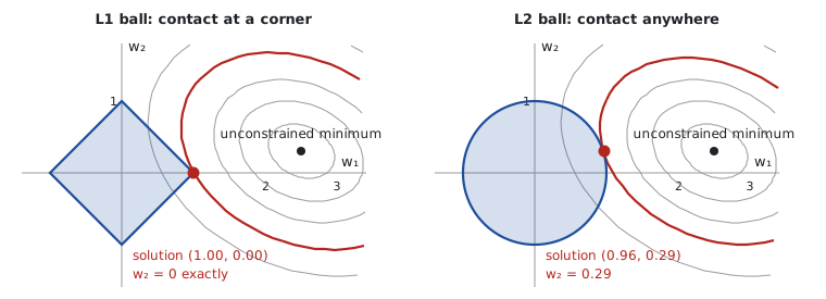
• The $L_2$ ball is round: the ellipse can touch it anywhere, and there’s no reason for that to be exactly on an axis. The weights are pulled toward 0 but stay non-zero.
• The $L_1$ ball has corners on the axes, i.e. where one coordinate is exactly 0. A growing ellipse is very likely to hit a corner before an edge. In the figure, the free minimum is at $(2.5, 0.3)$ : $w_2$ isn’t zero without the constraint, yet the $L_1$ solution sets it exactly to 0.

In high dimension, the effect gets stronger: the diamond becomes a polytope whose vertices and edges live on subspaces where many coordinates are zero. Hence sparse models: few non-zero weights.

5. The same result with calculus: soft thresholding versus division

Intuition. Look at the slope of each penalty near 0. The slope of $\frac{\lambda}{2} w^2$ is $\lambda w$ : it fades as $w$ approaches 0, so the slightest signal in the data is enough to keep a small weight. The slope of $\lambda|w|$ is $\pm\lambda$ : it pushes toward 0 with a constant force. If the data pull less hard than $\lambda$ , the weight stays exactly at 0.

In one dimension, with $z$ the least squares solution, we minimize $\frac{1}{2}(w - z)^2$ plus the penalty:

$$\begin{aligned} L_2 :\quad \hat w &= \frac{z}{1 + \lambda} \\ L_1 :\quad \hat w &= \operatorname{sign}(z)\, \max\big(|z| - \lambda,\ 0\big) \end{aligned}$$

For $L_1$ , the absolute value isn’t differentiable at 0: we use its subgradient, the interval $[-1, 1]$ . The optimality condition at $w = 0$ becomes $0 \in -z + \lambda\,[-1, 1]$ , i.e. $|z| \le \lambda$ . That’s soft thresholding: everything below the threshold $\lambda$ drops to zero, the rest is trimmed by $\lambda$ . $L_2$ divides everything by the same factor and zeroes nothing.

This formula is exact in several dimensions when the features are orthogonal ( $X^\top X / n = I$ ). In general, it’s the basic step of the algorithms that solve the Lasso (coordinate descent, proximal gradient).

A practical consequence: standardize. The penalty treats every weight the same way. A feature in milliseconds has a tiny weight, barely penalized; the same feature in seconds would have a weight 1,000 times larger, crushed by the penalty. Without standardization, regularization depends on units: always standardize first (M1, part 14).

6. Overview: SVMs and support vectors

A linear SVM looks for the hyperplane that separates the classes with the largest margin. It’s a constrained problem: minimize $\frac{1}{2}\|w\|^2$ subject to $y_i\,(w^\top x_i + b) \ge 1$ for every example $i$ , with $y_i \in \{-1, +1\}$ . Each constraint has its multiplier $\alpha_i \ge 0$ , and KKT complementary slackness says:

• examples far from the boundary have an inactive constraint, so $\alpha_i = 0$ : they don’t influence the solution;
• only examples on the margin have $\alpha_i > 0$ . These are the support vectors, and $w = \sum_i \alpha_i y_i x_i$ depends on them alone.

The KKT conditions therefore explain why an SVM boils down to a few examples. Exercise 4 checks it.

7. Weight decay and AdamW

With the penalty $\frac{\lambda}{2}\|\theta\|^2$ , the gradient gains a $\lambda\theta$ term and M10’s update becomes:

$$\theta_{t+1} = (1 - \eta\lambda)\,\theta_t - \eta\,\nabla L(\theta_t)$$

At every step, the weights are multiplied by a factor slightly below 1: that’s weight decay. With SGD, the $L_2$ penalty and weight decay are identical. With Adam, they aren’t: if you add $\lambda\theta$ to the gradient, it goes through the division by $\sqrt{\hat v_t}$ , and weights with large gradients barely shrink. AdamW (Loshchilov and Hutter, 2019) applies the $(1 - \eta\lambda)$ factor separately, after the Adam step: it’s the default optimizer for training the networks of part 22, the thesis LSTM included.

---

Code example

Lagrange in practice: the price of a constraint, and PCA

import numpy as np
from scipy.optimize import minimize

# 1. minimize f(x, y) = (x - 2)² + (y - 2)² subject to g(x, y) = x + 2y = c
f = lambda p: (p[0] - 2) ** 2 + (p[1] - 2) ** 2
grad_f = lambda p: np.array([2 * (p[0] - 2), 2 * (p[1] - 2)])
grad_g = np.array([1.0, 2.0])


def optimum(c):
    constraint = {"type": "eq", "fun": lambda p: p[0] + 2 * p[1] - c}
    return minimize(f, x0=np.zeros(2), constraints=[constraint], method="SLSQP", tol=1e-12).x


p = optimum(2.0)
lam = -(grad_f(p) @ grad_g) / (grad_g @ grad_g)      # ∇f + λ∇g = 0  =>  λ
print(f"optimum = {p.round(4)} | f = {f(p):.4f} | ∇f = {grad_f(p).round(4)} | λ = {lam:.4f}")
print(f"residual ∇f + λ∇g = {(grad_f(p) + lam * grad_g).round(8)}")
for c in (2.01, 2.1):                                # λ = price of the constraint
    print(f"c = {c}: f* = {f(optimum(c)):.4f} | change {f(optimum(c)) - f(p):+.4f} "
          f"| prediction -λ·Δc = {-lam * (c - 2):+.4f}")

# 2. PCA is a Lagrange problem: max wᵀCw subject to wᵀw = 1
rng = np.random.default_rng(0)
z = rng.normal(size=(500, 2)) * [3.0, 0.5]           # M3's cloud
R = np.array([[np.cos(0.6), -np.sin(0.6)], [np.sin(0.6), np.cos(0.6)]])
X = z @ R.T + [5.0, 2.0]
C = np.cov(X, rowvar=False)
unit_norm = {"type": "eq", "fun": lambda w: w @ w - 1}
w = minimize(lambda w: -w @ C @ w, x0=np.array([1.0, 0.0]), constraints=[unit_norm],
             method="SLSQP", tol=1e-12).x
print(f"w* = {w.round(4)} | multiplier wᵀCw = {w @ C @ w:.4f} | ‖Cw − λw‖ = {np.linalg.norm(C @ w - (w @ C @ w) * w):.1e}")
vals, vecs = np.linalg.eigh(C)
print(f"eigh: largest eigenvalue {vals[-1]:.4f}, vector {vecs[:, -1].round(4)}")

• The solver finds the optimum $(1.2, 0.4)$ with $f = 3.2$ and $\nabla f = (-1.6, -3.2)$ , exactly $-1.6 \times \nabla g$ : $\lambda = 1.6$ , as by hand.
• The price of the constraint: going from $c = 2$ to $c = 2.01$ , $f^*$ drops by $0.0160$ , exactly $\lambda \times 0.01$ . For $c = 2.1$ , the drop is $0.1580$ versus $0.1600$ predicted: the prediction is first-order, it drifts a little as $\Delta c$ grows.
• PCA: the constrained maximum is $w^* = (0.8247, 0.5656)$ , with a multiplier of $8.7383$ . That’s the largest eigenvalue of the covariance (M3’s $8.74$ ) and its eigenvector, up to sign.

The geometry, in numbers

This script computes the two contact points of the figure in section 4: a quadratic loss with minimum $(2.5, 0.3)$ , constrained to a ball of radius 1.

import numpy as np
from scipy.optimize import minimize

A = np.array([[1.0, 0.3], [0.3, 1.5]])
w0 = np.array([2.5, 0.3])                            # unconstrained minimum
loss = lambda w: (w - w0) @ A @ (w - w0)             # level sets = ellipses centered on w0
t = 1.0                                              # radius of the ball

balls = {
    "L1 (diamond)": {"type": "ineq", "fun": lambda w: t - np.abs(w).sum()},
    "L2 (circle) ": {"type": "ineq", "fun": lambda w: t - np.sqrt(w @ w)},
}
for name, constraint in balls.items():
    best = min((minimize(loss, x0=x0, constraints=[constraint], method="SLSQP", tol=1e-12)
                    for x0 in ([0.1, 0.1], [0.5, -0.4], [-0.3, 0.6])), key=lambda r: r.fun)
    w = best.x
    print(f"{name:<13} w* = ({w[0]:.4f}, {w[1]:.4f}) | loss = {best.fun:.4f} | gradient = {(2 * A @ (w - w0)).round(3)}")

Ball	Solution $w^*$	Loss	Loss gradient at $w^*$
$L_1$ (diamond)	$(1.0000, 0.0000)$	2.6550	$(-3.18, -1.80)$
$L_2$ (circle)	$(0.9561, 0.2930)$	2.3901	$(-3.092, -0.947)$

The $L_1$ solution lands exactly on the corner $(1, 0)$ . The $L_2$ solution keeps $w_2 = 0.29$ , and its gradient is indeed parallel to $w^*$ : $3.092 / 0.9561 \approx 0.947 / 0.2930 \approx 3.23$ . That’s the Lagrange condition, since the gradient of $\|w\|_2$ points in the direction of $w$ . For $L_1$ , the gradient isn’t parallel to the normal of an edge: at a corner, the ball has no unique normal, and that’s precisely what lets the solution stop there.

Soft thresholding, KKT conditions and penalty/constraint equivalence

We build 5 orthogonal features ( $X^\top X / n = I$ ) so that the formulas of section 5 are exact, with true weights $(3, -2, 1, 0.5, 0)$ .

import numpy as np
from scipy.optimize import minimize
from sklearn.linear_model import Lasso, Ridge

rng = np.random.default_rng(0)
n = 200
Q, _ = np.linalg.qr(rng.normal(size=(n, 5)))
X = Q * np.sqrt(n)                                   # orthogonal columns: XᵀX / n = I
w_true = np.array([3.0, -2.0, 1.0, 0.5, 0.0])
y = X @ w_true + rng.normal(0, 1, n)

z = X.T @ y / n                                      # least squares (since XᵀX / n = I)
lam = 0.8
soft = np.sign(z) * np.maximum(np.abs(z) - lam, 0)   # L1 solution: soft thresholding
shrunk = z / (1 + lam)                                    # L2 solution: plain division
lasso = Lasso(alpha=lam, fit_intercept=False).fit(X, y).coef_
ridge = Ridge(alpha=n * lam, fit_intercept=False).fit(X, y).coef_   # Ridge doesn't divide by n
print("least squares  :", z.round(3))
print("L1 (formula)   :", soft.round(3), "| sklearn Lasso :", lasso.round(3))
print("L2 (formula)   :", shrunk.round(3), "| sklearn Ridge :", ridge.round(3))

# Lasso KKT conditions: |Xᵀ(y − Xw)/n| = λ on non-zero weights, ≤ λ on zero weights
corr = X.T @ (y - X @ lasso) / n
print("|Xᵀr/n| :", np.abs(corr).round(3), "| zero weights:", np.isclose(lasso, 0))

# penalty <=> constraint: solve min (1/2n)‖y − Xw‖² subject to ‖w‖₁ ≤ t, with t = ‖w_lasso‖₁
t = np.abs(lasso).sum()
loss = lambda uv: np.sum((y - X @ (uv[:5] - uv[5:])) ** 2) / (2 * n)   # w = u − v, u, v ≥ 0
res = minimize(loss, x0=np.zeros(10), method="SLSQP", bounds=[(0, None)] * 10,
               constraints=[{"type": "ineq", "fun": lambda uv: t - uv.sum()}], tol=1e-12)
w_constrained = res.x[:5] - res.x[5:]
print(f"t = {t:.3f} | constrained solution: {w_constrained.round(3)} | max gap with the Lasso {np.abs(w_constrained - lasso).max():.1e}")

	$w_1$	$w_2$	$w_3$	$w_4$	$w_5$
True weights	3	−2	1	0.5	0
Least squares $z$	2.946	−1.923	0.971	0.455	−0.106
$L_1$ , $\lambda = 0.8$ (formula = scikit-learn)	2.146	−1.123	0.171	0	0
$L_2$ , $\lambda = 0.8$ (formula = scikit-learn)	1.637	−1.069	0.539	0.253	−0.059

What we read:

• the formulas of section 5 match scikit-learn to the thousandth. Watch the conventions: Lasso divides the loss by $2n$ , Ridge doesn’t, hence alpha=n * lam;
• $L_1$ trims every weight by exactly 0.8 and zeroes those that were below the threshold ( $0.455$ and $-0.106$ ). $L_2$ divides everything by 1.8 and zeroes nothing;
• the flip side: $L_1$ also removed $w_4$ , whose true weight is 0.5. A real but weak effect looks like noise. And the kept weights are biased toward 0: in practice, you often refit an unregularized model on the selected features;
• the KKT conditions show up in the correlation between the features and the residual: it’s exactly $0.8 = \lambda$ on the three non-zero weights (an “active” constraint for each), and stays below $\lambda$ ( $0.455$ and $0.106$ ) on the two zero weights;
• penalty = constraint: imposing $\|w\|_1 \le t$ with $t = 3.440$ (the norm of the Lasso solution), we recover the same solution to within $3.5 \times 10^{-8}$ . The Lasso’s $\lambda = 0.8$ is the multiplier of that constraint.

Running project: a regularization path to choose features

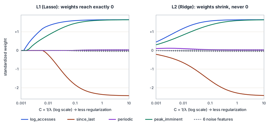
We reuse the synthetic memory regions from M9 and M10, with the 4 domain features, and add 6 pure-noise features. A good model should ignore them. We vary the regularization from very strong to almost none and track every weight: that’s the regularization path. In scikit-learn, the parameter is $C = 1/\lambda$ .

import numpy as np
from sklearn.linear_model import LogisticRegression
from sklearn.metrics import f1_score, log_loss
from sklearn.model_selection import train_test_split


def make_regions(n, rng):
    """Synthetic memory regions (same generator as M9 and M10): label 1 = hot in the next window."""
    rate = rng.gamma(0.6, 4, n)
    recent_accesses = rng.poisson(rate)
    since_last = np.round(rng.exponential(30 / (1 + recent_accesses)), 1)
    periodic = rng.binomial(1, 0.25, n)
    before_peak = rng.integers(0, 12, n)
    logit = (0.9 * np.log1p(recent_accesses) - 0.05 * since_last
             + 3.0 * periodic * (before_peak < 3) - 1.5 + rng.normal(0, 0.8, n))
    X = np.column_stack([recent_accesses, since_last, periodic, before_peak])
    return X, (logit > 0).astype(int)


def domain_features(X):
    return np.column_stack([np.log1p(X[:, 0]), X[:, 1], X[:, 2], X[:, 2] * (X[:, 3] < 3)])


rng = np.random.default_rng(0)
X, y = make_regions(5000, rng)
Xtr, Xte, ytr, yte = train_test_split(X, y, test_size=0.3, random_state=0, stratify=y)
# 4 useful features + 6 pure-noise features the model should ignore
names = ["log_accesses", "since_last", "periodic", "peak_imminent"] + [f"noise_{k}" for k in range(1, 7)]
Ftr = np.column_stack([domain_features(Xtr), rng.normal(size=(len(Xtr), 6))])
Fte = np.column_stack([domain_features(Xte), rng.normal(size=(len(Xte), 6))])
mu, sd = Ftr.mean(axis=0), Ftr.std(axis=0)
Ztr, Zte = (Ftr - mu) / sd, (Fte - mu) / sd          # standardize: the penalty must treat every weight alike

Cs = np.logspace(-3, 1, 41)                          # C = 1/λ: small C = strong regularization
paths = {}
for penalty, l1_ratio in (("l1", 1.0), ("l2", 0.0)):
    coefs = []
    for C in Cs:
        m = LogisticRegression(C=C, l1_ratio=l1_ratio, solver="saga", max_iter=20_000, tol=1e-8).fit(Ztr, ytr)
        coefs.append(m.coef_[0])
        if C in Cs[[0, 8, 16, 24, 40]]:
            p = m.predict_proba(Zte)[:, 1]
            print(f"{penalty} C = {C:<7.3g} non-zero weights = {np.sum(np.abs(m.coef_[0]) > 1e-6):>2} | "
                  f"‖w‖₁ = {np.abs(m.coef_[0]).sum():6.3f} | test log loss = {log_loss(yte, p):.4f} | "
                  f"test F1 = {f1_score(yte, (p > 0.5).astype(int)):.3f}")
    paths[penalty] = np.array(coefs)

# order in which features enter the L1 path (smallest C where the weight becomes non-zero)
entry = [Cs[np.argmax(np.abs(paths["l1"][:, j]) > 1e-6)] if (np.abs(paths["l1"][:, j]) > 1e-6).any()
          else np.inf for j in range(len(names))]
for j in np.argsort(entry):
    print(f"  {names[j]:<15} enters at C = {entry[j]:.3g} | weight at C = 10: L1 {paths['l1'][-1, j]:+.3f}, L2 {paths['l2'][-1, j]:+.3f}")
print("smallest |L2 weight| along the whole path:", f"{np.abs(paths['l2']).min():.1e}")

Penalty	$C$	Non-zero weights (out of 10)	$\lVert w \rVert_1$	Test log loss	Test F1
$L_1$	0.001	0	0.000	0.5278	0.000
$L_1$	0.0063	2	1.816	0.3309	0.575
$L_1$	0.040	3	4.058	0.2921	0.681
$L_1$	0.25	9	5.522	0.2884	0.680
$L_1$	10	10	5.967	0.2884	0.685
$L_2$	0.001	10	1.110	0.3921	0.289
$L_2$	0.040	10	4.070	0.2933	0.679
$L_2$	10	10	5.957	0.2884	0.685

Order of entry into the $L_1$ path: log_accesses ( $C = 0.0016$ ), peak_imminent ( $0.002$ ), since_last ( $0.0079$ ), then a first noise feature at $C = 0.050$ , and periodic only at $C = 0.1$ .

What the path shows:

• under very strong regularization, $L_1$ zeroes everything. The model then predicts the base rate (log loss 0.528, F1 zero). $L_2$ , at the same $C$ , keeps all 10 weights non-zero: along the whole path, the smallest $L_2$ weight is $1.6 \times 10^{-5}$ , never exactly 0;
• at $C = 0.04$ , $L_1$ keeps only 3 features out of 10, and they’re the right ones: log_accesses, peak_imminent and since_last. With them alone, the test F1 is 0.681, versus 0.685 for the full model. The 6 noise features brought nothing;
• periodic enters after the first noise feature, and its final weight stays tiny (+0.03). That’s correct: in the generator, being periodic only matters as the peak approaches, and that information is already in peak_imminent. The $L_1$ path recovered the structure of the problem without being told;
• without regularization ( $C = 10$ ), $L_1$ and $L_2$ give the same model: when the ball is large enough to contain the free minimum, the constraint is inactive ( $\mu = 0$ ), whatever its shape.

To choose $C$ for real, you don’t look at the test set: you cross-validate along the path (LogisticRegressionCV, part 18). The path itself is for understanding which features carry the signal.

---

Hands-on exercise

1. By hand. Maximize $f(x, y) = xy$ subject to $x + y = 10$ with a Lagrange multiplier. Then check the interpretation of $\lambda$ as the price of the constraint: how much does the maximum increase when you move to $x + y = 10.1$ ?
2. Soft thresholding. Derive the formula $\operatorname{sign}(z)\max(|z| - \lambda, 0)$ by handling the cases $w > 0$ , $w < 0$ and $w = 0$ separately. Then, on the example’s orthogonal features, count the Lasso’s zero weights for $\lambda \in \{0.1, 0.5, 1, 2, 3\}$ , predicting the result before running the code.
3. Correlated features. In the running project, add a noisy copy of log_accesses (the same column plus noise with standard deviation 0.05). Compare the weights of the two copies with $L_1$ and with $L_2$ at $C = 0.04$ . Which one spreads the weight, which one picks a copy? Then try the elastic net with l1_ratio=0.5.
4. SVM and KKT. Train SVC(kernel="linear", C=1.0) on the running project’s 4 standardized domain features (2,000 examples are enough). How many support vectors (support_)? Check that examples with $y_i f(x_i) > 1$ (computed with decision_function and $y_i \in \{-1, +1\}$ ) are never support vectors.
5. Adam versus AdamW. In M10’s Adam trainer, on the raw features, add regularization in two ways: $\lambda w$ added to the gradient before Adam, then the $(1 - \eta\lambda)$ factor applied after the step (AdamW), with $\lambda = 0.01$ . Which weight shrinks the most in each case? Relate the answer to the scale of since_last.
6. Running project. On the 9 features of part 14, plot the $L_1$ path. Which features enter first? Which ones only enter under weak regularization? Compare with the feature importances of part 19.

Hint for question 1: the optimum is $(5, 5)$ with $\lambda = 5$ . For $x + y = c$ , the maximum is $c^2/4$ : it goes from 25 to 25.5025, i.e. about $5 \times 0.1$ .

---

Further resources

• James, Witten, Hastie and Tibshirani, An Introduction to Statistical Learning (ISLR), chapter 6, section 6.2: Ridge, Lasso and the balls figure, free online.
• Hastie, Tibshirani and Friedman, The Elements of Statistical Learning, section 3.4: shrinkage methods and regularization paths.
• Tibshirani, Regression Shrinkage and Selection via the Lasso (Journal of the Royal Statistical Society B, 1996): the paper that introduced the Lasso.
• Boyd and Vandenberghe, Convex Optimization, chapter 5 (duality and KKT conditions), free online.
• Bishop, Pattern Recognition and Machine Learning, appendix E (Lagrange multipliers) and chapter 7 (SVMs).
• Loshchilov and Hutter, Decoupled Weight Decay Regularization (ICLR 2019): AdamW.

---

What you should be able to do before moving on

• Solve a simple problem with a Lagrange multiplier and interpret $\lambda$ as the price of the constraint
• Write the KKT conditions and say whether a constraint is active or inactive
• Explain why a penalty $\lambda\|\theta\|$ is equivalent to a constraint $\|\theta\| \le t$
• Explain geometrically why $L_1$ zeroes weights and $L_2$ shrinks them
• Derive soft thresholding and the $1/(1 + \lambda)$ factor
• Read a regularization path and explain why you standardize before regularizing
• Say what AdamW changes compared with an $L_2$ penalty inside Adam

Next part: M12 · Wrap-up: rereading everything with the maths. We go back over the whole maths programme and tie it to the models of the technical phase, from the dot product to the thesis LSTM.