M3 · Eigenvalues, SVD and PCA

Mastering AI · Required Maths · Week 1 (linear algebra) · Part 3

Goal of this step

M2 showed that a matrix skews space. This article answers the next question: are there directions the matrix doesn’t skew, that it only stretches? The answer yields three tools we’ll use everywhere:

• eigenvalues and eigenvectors, which describe a matrix by its preferred directions;
• the SVD, which breaks any matrix into rotation, stretch, rotation;
• PCA, which follows directly and reduces the dimension of data while keeping most of its variance.

By the end of this article you’ll be able to code a PCA from scratch, interpret explained variance, and know what PCA can and cannot see in memory access profiles.

---

Key concepts

1. Eigenvectors: the directions that don’t turn

Intuition. Apply a matrix to every vector in the plane. Most change direction. A few special directions are only lengthened, shortened or flipped: those are the eigen-directions, and the stretch factor is the eigenvalue.

$$A v = \lambda v, \qquad v \neq 0$$

• $\lambda > 1$ : the direction is stretched; $0 < \lambda < 1$ : shrunk; $\lambda < 0$ : flipped; $\lambda = 0$ : squashed (it’s in the null space, M2).
• The determinant is the product of the eigenvalues: $\det A = \prod_i \lambda_i$ . That’s consistent with M2’s volume factor: we multiply the stretch of each direction.

Why it’s useful. In the eigenvector basis, the matrix becomes diagonal: just a list of independent stretches. Applying $A$ a hundred times means raising each $\lambda$ to the 100th power. Directions with $|\lambda| > 1$ blow up and those with $|\lambda| < 1$ vanish. That’s exactly the mechanism behind exploding and vanishing gradients in an RNN, where the same matrix is applied at every time step (part 23).

2. Symmetric matrices

Intuition. Symmetric matrices ( $A = A^\top$ ) are the nicest: they stretch space along perpendicular axes, with no shearing. A circle becomes an ellipse whose axes are the eigenvectors.

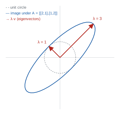
In this figure, the matrix $A = \begin{pmatrix} 2 & 1 \\ 1 & 2 \end{pmatrix}$ stretches the diagonal direction by 3 and leaves the perpendicular direction untouched. Those two directions are exactly the ellipse’s axes.

Spectral theorem. A real symmetric matrix has real eigenvalues and orthogonal eigenvectors. So it can be written:

$$A = Q \Lambda Q^\top$$

with $Q$ orthogonal (its columns are the unit eigenvectors) and $\Lambda$ diagonal (the eigenvalues). Read right to left: rotate to align with the eigen-axes ( $Q^\top$ ), stretch each axis ( $\Lambda$ ), rotate back ( $Q$ ).

Symmetric matrices are everywhere in ML: the data’s covariance matrix, $X^\top X$ in least squares, and the Hessian of a loss function (M6).

3. The SVD: the universal decomposition

Intuition. The spectral theorem only works for square symmetric matrices. The SVD extends the idea to any matrix, even rectangular: every linear transformation is a rotation, then a stretch along the axes, then another rotation.

$$A = U \Sigma V^\top$$

• $V^\top$ : a rotation in the input space;
• $\Sigma$ : a stretch along the axes by the singular values $\sigma_1 \ge \sigma_2 \ge \dots \ge 0$ ;
• $U$ : a rotation in the output space.

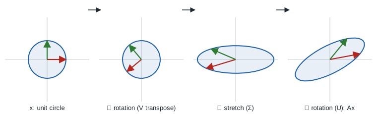
The red and green arrows track $e_1$ and $e_2$ through each step. The rotation $V^\top$ distorts nothing; all the flattening comes from $\Sigma$ ; the rotation $U$ orients the result. Together, the three steps give exactly the effect of $A$ .

The rank of $A$ is the number of non-zero singular values. The link with what came before: the singular values of $A$ are the square roots of the eigenvalues of $A^\top A$ , and the columns of $V$ are its eigenvectors.

Rank- $k$ approximation. $A$ can be written as a sum of rank-1 matrices, ordered by importance:

$$A = \sum_{i} \sigma_i\, u_i v_i^\top \qquad\Longrightarrow\qquad A_k = \sum_{i=1}^{k} \sigma_i\, u_i v_i^\top$$

Keeping the first $k$ terms gives the best possible rank- $k$ approximation (Eckart-Young theorem). That’s the basis of compression, PCA and recommender systems.

4. PCA, derived from all this

Intuition. Your point cloud lives in $\mathbb{R}^d$ , but it’s often “flattened”: it spreads a lot in some directions and very little in others. PCA finds the directions where the data varies most, then projects onto them.

In three steps:

1. Center the data: $X_c = X - \bar x$ .
2. Compute the covariance matrix $C = \frac{1}{n-1} X_c^\top X_c$ . It’s symmetric, so diagonalizable with orthogonal axes.
3. Its eigenvectors are the principal components, and its eigenvalues are the variances along each component → see M7 for covariance.

In practice we don’t even compute $C$ : we take the SVD of $X_c$ directly. The rows of $V^\top$ are the components, and the variance of component $i$ is $\sigma_i^2 / (n-1)$ . It’s more numerically stable.

Explained variance. The share of variance captured by component $i$ is:

$$\frac{\lambda_i}{\sum_j \lambda_j}$$

If the first two components capture 95% of the variance, the data can be shown in 2D with little information lost.

Limits to keep in mind:

• PCA only sees linear structure and directions of variance; a highly predictive but low-variance variable can be discarded;
• it’s scale-sensitive: standardize features first (M1);
• the sign of a component is arbitrary: $v$ and $-v$ are the same direction.

---

Code example

Eigenvectors of a symmetric matrix

This script reproduces the figure from section 2.

import numpy as np
import matplotlib.pyplot as plt

A = np.array([[2.0, 1.0],
              [1.0, 2.0]])                  # symmetric
values, vectors = np.linalg.eigh(A)         # eigh: for symmetric matrices
print("eigenvalues:", values)
print("eigenvectors (columns):\n", vectors.round(4))
for lam, v in zip(values, vectors.T):
    print(f"A v = {A @ v} ; lambda v = {lam * v}")
print("orthogonal?", np.isclose(vectors[:, 0] @ vectors[:, 1], 0))

theta = np.linspace(0, 2 * np.pi, 200)
circle = np.stack([np.cos(theta), np.sin(theta)])
ellipse = A @ circle
fig, ax = plt.subplots(figsize=(5, 5))
ax.plot(*circle, c="lightgray", label="unit circle")
ax.plot(*ellipse, c="tab:blue", label="image under A")
for lam, v in zip(values, vectors.T):
    ax.arrow(0, 0, *(lam * v), color="tab:red", width=0.03, length_includes_head=True)
ax.set_aspect("equal")
ax.legend()
ax.set_title("The ellipse's axes are the eigenvectors")
plt.show()

The eigenvalues are $1$ and $3$ , for directions $(-1, 1)/\sqrt 2$ and $(1, 1)/\sqrt 2$ , which are orthogonal. Check: $\det A = 2 \times 2 - 1 \times 1 = 3 = 1 \times 3$ .

A PCA by hand, compared with scikit-learn

We build an elongated 2D cloud, rotated and shifted, then recover its axes.

import numpy as np
from sklearn.decomposition import PCA

rng = np.random.default_rng(0)
n = 500
z = rng.normal(size=(n, 2)) * [3.0, 0.5]                   # lots of variance on one axis
R = np.array([[np.cos(0.6), -np.sin(0.6)], [np.sin(0.6), np.cos(0.6)]])
X = z @ R.T + [5.0, 2.0]                                    # rotated and shifted

Xc = X - X.mean(axis=0)                                     # 1. center
U, S, Vt = np.linalg.svd(Xc, full_matrices=False)           # 2. SVD
components = Vt                                             # principal directions (rows)
explained_variance = S**2 / (n - 1)
ratio = explained_variance / explained_variance.sum()
print("PCA by hand: components\n", components.round(4), "\nratio:", ratio.round(4))

pca = PCA().fit(X)
print("sklearn PCA: components\n", pca.components_.round(4),
      "\nratio:", pca.explained_variance_ratio_.round(4))

C = np.cov(Xc, rowvar=False)
val_c, vec_c = np.linalg.eigh(C)
print("covariance eigenvalues:", val_c[::-1].round(4),
      "| S^2/(n-1):", explained_variance.round(4))

What we see:

• the first component captures 97.4% of the variance, as expected for an almost one-dimensional cloud;
• the direction found, $(0.8247,\ 0.5656)$ , matches the 0.6 radian rotation used to build the data ( $\cos 0.6 \approx 0.825$ , $\sin 0.6 \approx 0.565$ );
• our version and scikit-learn’s have opposite signs: that’s fine, it’s the same direction;
• the covariance eigenvalues ( $8.74$ and $0.23$ ) are exactly $\sigma_i^2/(n-1)$ : covariance and SVD say the same thing.

What PCA sees in memory access profiles

We reuse the idea from M1: each region is described by its accesses over 50 aggregations, a point in $\mathbb{R}^{50}$ . We generate 400 profiles of four types.

import numpy as np
import matplotlib.pyplot as plt
from sklearn.decomposition import PCA

rng = np.random.default_rng(0)


def profile(kind, rng, L=50):
    t = np.arange(L)
    if kind == "periodic":
        period = rng.integers(8, 15)
        return (((t + rng.integers(0, period)) % period) < 2) * rng.uniform(3, 8)
    if kind == "hot":
        return rng.poisson(rng.uniform(2, 6), L).astype(float)
    if kind == "cold":
        return rng.poisson(0.05, L).astype(float)
    # burst: a single period of intense activity
    start = rng.integers(0, L - 10)
    x = np.zeros(L)
    x[start:start + rng.integers(5, 10)] = rng.uniform(4, 8)
    return x


kinds = ["periodic", "hot", "cold", "burst"]
labels = rng.choice(kinds, size=400)
P = np.array([profile(k, rng) for k in labels])

pca_p = PCA(n_components=10).fit(P)
print("explained variance per component:", pca_p.explained_variance_ratio_.round(3))
print("cumulative:", np.cumsum(pca_p.explained_variance_ratio_).round(3))
print("component 1 (start):", pca_p.components_[0, :10].round(3))

Z = pca_p.transform(P)[:, :2]
fig, ax = plt.subplots(figsize=(6, 5))
for k in kinds:
    m = labels == k
    ax.scatter(Z[m, 0], Z[m, 1], s=10, label=k)
ax.set_xlabel("component 1")
ax.set_ylabel("component 2")
ax.legend()
ax.set_title("400 profiles from R^50 projected to 2D")
plt.show()

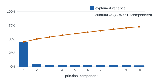
Results:

• component 1 captures 45% of the variance. Its coefficients are all positive and nearly equal (around 0.14): it’s simply the profile’s overall intensity. On the scatter plot, it cleanly separates cold regions (left) from hot ones (right);
• component 2 captures only 5%. It spreads bursts according to whether they come early or late in the window;
• beyond that, variance is scattered: 10 components explain only 72% of the total;
• periodic profiles overlap with bursts. PCA can’t tell them apart.

The last point is the most instructive. As in M1, periodic profiles have random phases: two regions with the same rhythm but shifted are nearly orthogonal vectors. So there’s no single direction in $\mathbb{R}^{50}$ that represents “being periodic”, and a linear method can’t find what isn’t a direction. The fix is the same: build shift-invariant features (period, phase, autocorrelation) before any analysis. We’ll redo this PCA in part 20, on the part 14 features rather than raw profiles.

Compressing an image with a truncated SVD

A grayscale image is a matrix. Its truncated SVD gives the best rank- $k$ approximation.

import numpy as np
import matplotlib.pyplot as plt
from sklearn.datasets import load_sample_image

img = load_sample_image("china.jpg").mean(axis=2)   # grayscale, 427 x 640
U, S, Vt = np.linalg.svd(img, full_matrices=False)

ranks = [5, 20, 50, 100]
fig, axes = plt.subplots(1, len(ranks) + 1, figsize=(18, 3.5))
axes[0].imshow(img, cmap="gray")
axes[0].set_title(f"original (rank {np.linalg.matrix_rank(img)})")
for ax, k in zip(axes[1:], ranks):
    approx = U[:, :k] @ np.diag(S[:k]) @ Vt[:k]
    error = np.linalg.norm(img - approx) / np.linalg.norm(img)
    size = k * (img.shape[0] + img.shape[1] + 1) / img.size
    ax.imshow(approx, cmap="gray")
    ax.set_title(f"rank {k}: error {error:.1%}, size {size:.0%}")
    print(f"rank {k:>3}: relative error = {error:.3f}, size = {size:.3f}")
for ax in axes:
    ax.axis("off")
plt.tight_layout()
plt.show()

Rank $k$	Relative error	Stored size
5	18.4%	2%
20	13.6%	8%
50	10.3%	20%
100	7.4%	39%

For rank $k$ we store $k$ columns of $U$ , $k$ rows of $V^\top$ and $k$ singular values, i.e. $k(m + n + 1)$ numbers instead of $mn$ . At rank 50 we keep 20% of the numbers for a perfectly recognizable image.

---

Hands-on exercise

1. By hand. Compute the eigenvalues of $A = \begin{pmatrix} 4 & 1 \\ 2 & 3 \end{pmatrix}$ by solving $\det(A - \lambda I) = 0$ . Check with np.linalg.eig. Are the eigenvectors orthogonal? Why?
2. Matrix powers. With the example’s symmetric matrix, compute $A^{10} x$ for several random vectors $x$ and normalize the result. Which direction do they all converge to? That’s the power iteration method. Explain why it works using diagonalization.
3. Scale matters. In the 2D PCA, multiply the second column of X by 100 before the PCA. What happens to the first component? Redo it after StandardScaler. Which analysis makes sense?
4. PCA on features. Take the part 14 dataset (or recompute the 9 features on this article’s profiles). Apply StandardScaler then a PCA. How many components for 90% of the variance? Do periodic profiles separate from bursts better than on raw profiles?
5. Least squares via SVD. With $X = U \Sigma V^\top$ , show that the least squares solution is $\hat w = V \Sigma^{-1} U^\top y$ . Implement it and compare with np.linalg.lstsq on M2’s example.

Hint for question 2: write $x$ in the eigenvector basis, $x = c_1 v_1 + c_2 v_2$ . What is $A^{10} x$ ?

---

Further resources

• 3Blue1Brown, Essence of Linear Algebra, episode 14 (Eigenvectors and eigenvalues).
• Gilbert Strang, MIT 18.06, lectures 21, 25 and 29 (eigenvalues, symmetric matrices, SVD).
• Deisenroth et al., Mathematics for Machine Learning, chapter 4 (matrix decompositions) and chapter 10 (PCA).
• Jonathon Shlens, A Tutorial on Principal Component Analysis (2014), free on arXiv: PCA derived step by step.

---

What you should be able to do before moving on

• Explain an eigenvector with a drawing, without formulas
• Compute the eigenvalues of a $2 \times 2$ matrix by hand
• State the spectral theorem and say why covariance fits it
• Read the SVD as rotation, stretch, rotation, and use the rank- $k$ approximation
• Code a PCA with np.linalg.svd and interpret explained variance
• Name three limits of PCA (linearity, scale, variance isn’t relevance)

Next part: M4 · Derivatives, partial derivatives and the gradient. Calculus week starts: how a loss function changes when we move the parameters.