Sequence models: RNNs, LSTMs and attention

Mastering AI · Technical phase · Week 3 · Part 23

Goal of this step

Since part 14, every model has seen a region’s past through 9 hand-picked features: rolling means, time since the last access, estimated period. That’s a summary. A sequence model instead receives the raw sequence of accesses and builds its own memory. That’s hypothesis H2 of the thesis: does an LSTM on the raw history beat LightGBM or an MLP on features?

We’ll answer with the recipe from part 22 applied to every model, with the same budget, and then look at what each gain costs in latency.

By the end of this article you’ll be able to:

• turn a trace into windows $(x_{t-L+1}, \dots, x_t)$ ready for PyTorch, without leakage;
• explain why an RNN forgets fast, with the chain rule from M5, and what an LSTM’s gates change;
• use a dilated 1D convolution as a fast alternative to recurrence;
• write an attention head and connect its score to the dot product from M1;
• decide, with numbers, when a sequence model is worth its cost.

---

Key concepts

1. Shaping a series: windows

Intuition. To predict whether a region will be accessed within the next second, we show it the video of its last $L$ aggregations instead of the 9-feature summary sheet.

For each row (region $r$ , time $t$ ) of the dataset, the input becomes an $L \times 2$ matrix: at each time $s$ from $t-L+1$ to $t$ , the region’s number of accesses and the mean of its two neighbors (part 14’s locality). The label doesn’t change: $y_t = 1$ if the region is accessed between $t+1$ and $t+H$ , with $H = 10$ .

The three anti-leakage rules from part 14 apply as they are:

• the window stops at $t$ : never a later time step;
• log1p and standardization use statistics computed on the training period only;
• the split stays the one from part 15: train $t < 1390$ , validation $1400 \le t < 1790$ , test $t \ge 1800$ . The 10-aggregation gaps are the purge.

On the PyTorch side, a batch of sequences is a tensor of shape (batch, L, channels). Choosing $L$ is a real modeling choice: a window shorter than a region’s period cannot see its cycle.

2. The RNN: a memory that fades

Intuition. An RNN reads the window from left to right, the way you read a text, updating a summary $h$ (the hidden state) at each step. The same weights are used at every step.

$$h_s = \tanh\left(W_x x_s + W_h h_{s-1} + b\right), \qquad \hat y = \sigma\left(w^\top h_t + c\right)$$

To know how the input from $k$ steps ago influences the output, we apply M5’s chain rule along the recurrence:

$$\frac{\partial h_t}{\partial h_{t-k}} = \prod_{s=t-k+1}^{t} \operatorname{diag}\left(1 - h_s^2\right) W_h$$

It’s a product of $k$ matrices. If their “size” is below 1, it decreases geometrically with $k$ : that’s the vanishing gradient, the same chain of multiplications as part 22’s 16 layers, except that depth is now the window length. The RNN cannot learn a dependency 40 steps back if the error signal that travels back 40 steps is $10^{-8}$ . If the size exceeds 1, it explodes: that’s why we keep clip_grad_norm_ in the loop.

3. LSTM and GRU: gates to decide what to keep

Intuition. The LSTM adds a second memory, the cell $c$ , which isn’t multiplied by a matrix at each step: we add information to it, and gates decide what to forget.

$$\begin{aligned} f_s &= \sigma\left(W_f [h_{s-1}, x_s] + b_f\right) && \text{forget gate} \\ i_s &= \sigma\left(W_i [h_{s-1}, x_s] + b_i\right) && \text{input gate} \\ c_s &= f_s \odot c_{s-1} + i_s \odot \tanh\left(W_c [h_{s-1}, x_s] + b_c\right) \\ h_s &= o_s \odot \tanh(c_s) && o_s \text{: output gate} \end{aligned}$$

Along the cell, the derivative is simply $\partial c_s / \partial c_{s-1} = \operatorname{diag}(f_s)$ (ignoring the paths that go through $h$ ). After $k$ steps, what remains is the product of the forget gates: if $f \approx 1$ , information and gradient cross the window almost intact. The network learns when to forget.

A detail that matters, and that we’ll measure: at initialization, PyTorch sets all biases to small values centered on 0, so $f \approx \sigma(0) = 0.5$ , and $0.5^{40} \approx 10^{-12}$ . A brand-new LSTM forgets as fast as an RNN. Hence the classic trick (Jozefowicz et al., 2015): initialize the forget-gate bias $b_f$ to 1 or more.

The GRU (Cho et al., 2014) merges cell and hidden state and has only two gates: 25% fewer parameters, often similar results.

4. The 1D convolution: looking at the whole window at once

Intuition. Instead of reading the window step by step, we slide small filters along time, like a rolling mean whose weights are learned. All time steps are processed in parallel.

A size-3 filter only sees 3 time steps. To see far without stacking 30 layers, we dilate: layer $j$ looks at time steps spaced $d_j$ apart. With kernel $k$ and dilations $d_1, \dots, d_n$ , the receptive field is

$$R = 1 + (k - 1) \sum_{j=1}^{n} d_j$$

With $k = 3$ and $d = 1, 2, 4, 8, 16$ : $R = 1 + 2 \times 31 = 63$ . Five layers are enough to see 63 time steps. No recurrence, so no product of $k$ Jacobians: the gradient from a distant time step goes through 5 layers, not 63.

5. Attention: the query chooses whom to listen to

Intuition. To decide now, the present step asks a question (the query). Each past step shows a label (its key) and a content (its value). We mostly listen to the steps whose label resembles the question.

Each time step $s$ is first projected into a vector $z_s$ of dimension $d$ (here 32), to which we add a learned position vector. Then:

$$q = W_Q z_t, \quad k_s = W_K z_s, \quad v_s = W_V z_s, \qquad \alpha_s = \frac{\exp\left(q^\top k_s / \sqrt{d}\right)}{\sum_{u} \exp\left(q^\top k_u / \sqrt{d}\right)}, \qquad \text{context} = \sum_s \alpha_s v_s$$

The score $q^\top k_s$ is M1’s dot product: it’s large when the two vectors point in the same direction. Dividing by $\sqrt{d}$ keeps scores at a reasonable scale (the variance of a sum of $d$ independent products, M7); otherwise the softmax would saturate. The weights $\alpha_s$ are positive and sum to 1: we can read them, it’s one of the few models that tells you where it looks.

Without the position vectors, attention wouldn’t know the order: permuting the window would change nothing. This is the heart of Transformers; here, a single head and a single layer are enough to see the idea.

6. When is a sequence model worth its cost?

Intuition. A sequence model only learns what the window contains. If good features already summarize that past, it has to do better than them, not just as well, to justify a much higher cost.

Criterion	Features + MLP / boosting	Sequence model
What it sees	what you thought of computing, over long horizons (mean_100, since_last up to 500)	everything in the window, nothing beyond $L$
Inference cost	a few tens of µs	at least $L$ times more computation (recurrence: $L$ sequential steps)
Data needed	moderate	more parameters, more sensitive to tuning
When it wins	patterns that are easy to summarize	patterns nobody managed to summarize: precise order, temporal interactions

So the honest question isn’t “is the LSTM good?” but “what do we gain over part 22’s MLP, with equal tuning, and how many microseconds does it cost?”.

---

Code example

As in parts 15 to 22, we reuse part 14’s script as is (simulation and dataset), then the first block of part 22 (split, 9-feature inputs, mlp, evaluate, fit, range test), and add the four blocks below after them. The whole thing runs in about half an hour on a two-core CPU (numpy 2.5, pandas 3.0, scikit-learn 1.9, torch 2.14).

From features to sequences

We build the two channels once (the region’s accesses, the mean of its two neighbors), apply log1p and standardization with the statistics of time steps $t < 1390$ , then cut the windows with sliding_window_view, which copies nothing: each window is a view on the same memory.

# 1. From features to sequences: the raw window of the last L aggregations
from numpy.lib.stride_tricks import sliding_window_view

# Two channels per time step: the region's accesses, and the mean of its two neighbors (r-1, r+1)
neighbors = np.stack([accesses[[v for v in (r - 1, r + 1) if 0 <= v < N_REGIONS]].mean(0)
                     for r in range(N_REGIONS)])
channels = np.log1p(np.stack([accesses, neighbors], axis=-1)).astype(np.float32)   # (regions, time, 2)
mean = channels[:, :1390].reshape(-1, 2).mean(0)          # train statistics only (part 14)
scale = channels[:, :1390].reshape(-1, 2).std(0)
channels = (channels - mean) / scale


def sequences(d, L):
    """For each row (region, t): the L time steps t-L+1 .. t inclusive, never beyond t."""
    windows = sliding_window_view(channels, L, axis=1)      # (regions, T-L+1, 2, L), no copy
    X = windows[d.region.to_numpy(), d.t.to_numpy() - L + 1].transpose(0, 2, 1)
    return torch.tensor(np.ascontiguousarray(X))           # (n, L, 2)


S = {L: (sequences(tr, L), sequences(va, L), sequences(te, L)) for L in (20, 64)}
print(tuple(S[64][0].shape), tuple(S[64][1].shape), tuple(S[64][2].shape))
# Leakage check: the window's last step is indeed the row's time t
r0, t0_ = int(tr.region.iloc[5000]), int(tr.t.iloc[5000])
print("last step = accesses at t:", np.isclose(np.expm1(S[64][0][5000, -1, 0].item() * scale[0] + mean[0]),
                                                accesses[r0, t0_], atol=1e-3))

Output: (123840, 64, 2) (37440, 64, 2) (114240, 64, 2), then last step = accesses at t: True. Same rows as part 22’s 9 features, same labels: only the representation of the input changes. The check verifies the most important rule: the window’s last time step is exactly the row’s time $t$ , never $t+1$ .

Four ways to read a sequence, and memory at initialization

All four models take a (batch, L, 2) tensor and return a logit. Before any training, we measure the sensitivity of the output to the input from $k$ steps ago: the norm of $\partial \text{output} / \partial x_{t-k}$ over 512 windows, divided by the one at $k = 0$ . It’s the formula from section 2, measured.

# 2. Four ways to read a sequence
class Recurrent(nn.Module):
    """RNN, LSTM or GRU: read the window in order, predict from the last hidden state."""
    def __init__(self, cell="lstm", d_in=2, hidden=32, forget_bias=None):
        super().__init__()
        self.rnn = {"rnn": nn.RNN, "lstm": nn.LSTM, "gru": nn.GRU}[cell](d_in, hidden, batch_first=True)
        self.head = nn.Linear(hidden, 1)
        if forget_bias is not None:              # LSTM: biases are stored per gate [i, f, g, o]
            with torch.no_grad():
                self.rnn.bias_ih_l0[hidden:2 * hidden].fill_(forget_bias)
                self.rnn.bias_hh_l0[hidden:2 * hidden].zero_()

    def forward(self, x):                        # x : (batch, L, 2)
        states, _ = self.rnn(x)                  # (batch, L, hidden): one hidden state per step
        return self.head(states[:, -1])          # the last one summarizes the whole window -> a logit


class Conv1D(nn.Module):
    """Dilated convolutions 1, 2, 4, 8, 16 (kernel 3): a 63-step receptive field, no recurrence."""
    def __init__(self, d_in=2, c=32, dilations=(1, 2, 4, 8, 16)):
        super().__init__()
        layers, a = [], d_in
        for dil in dilations:
            layers += [nn.Conv1d(a, c, kernel_size=3, dilation=dil), nn.ReLU()]
            a = c
        self.convs = nn.Sequential(*layers)
        self.head = nn.Linear(c, 1)

    def forward(self, x):                        # Conv1d expects (batch, channels, L)
        z = self.convs(x.transpose(1, 2))        # no padding: L - 62 positions remain
        return self.head(z[:, :, -1])            # the last one sees the last 63 steps


class Attention(nn.Module):
    """One attention head: the present step (the query) chooses which past steps (the keys) to listen to."""
    def __init__(self, d_in=2, d=32, L=64):
        super().__init__()
        self.inp = nn.Linear(d_in, d)
        self.position = nn.Parameter(0.1 * torch.randn(L, d))     # without it, order would be lost
        self.attn = nn.MultiheadAttention(d, num_heads=1, batch_first=True)
        self.head = nn.Sequential(nn.Linear(2 * d, d), nn.ReLU(), nn.Linear(d, 1))

    def forward(self, x):
        z = self.inp(x) + self.position                      # (batch, L, d)
        q = z[:, -1:]                                           # query: time t
        context, self.weights = self.attn(q, z, z)              # weights: (batch, 1, L), sum to 1
        return self.head(torch.cat([context[:, 0], q[:, 0]], dim=-1))


def n_params(m):
    return sum(p.numel() for p in m.parameters())


# Memory at initialization: how much does the output depend on the input from k steps ago?
xb = S[64][0][:512].clone().requires_grad_()
for name, make in [("RNN", lambda: Recurrent("rnn")), ("LSTM", lambda: Recurrent("lstm")),
                      ("LSTM, forget bias 1", lambda: Recurrent("lstm", forget_bias=1.0)),
                      ("LSTM, forget bias 3", lambda: Recurrent("lstm", forget_bias=3.0))]:
    torch.manual_seed(0)
    m = make()
    xb.grad = None
    m(xb).sum().backward()
    g = xb.grad.norm(dim=(0, 2))                                # one norm per position
    print(f"{name:>20} | {n_params(m)} parameters | |d output / d x_(t-k)| relative to k = 0: "
          + " ".join(f"k={k}: {(g[-1 - k] / g[-1]).item():.1e}" for k in (1, 5, 10, 20, 40, 63)))

Model (initialization)	$k = 1$	$k = 5$	$k = 10$	$k = 20$	$k = 40$	$k = 63$
RNN (1,185 parameters)	0.16	0.10	$9.4 \times 10^{-3}$	$2.0 \times 10^{-4}$	$3.3 \times 10^{-8}$	$1.6 \times 10^{-12}$
LSTM (4,641 parameters)	0.59	$5.3 \times 10^{-2}$	$4.2 \times 10^{-3}$	$2.2 \times 10^{-5}$	$1.1 \times 10^{-9}$	$7.3 \times 10^{-14}$
LSTM, forget bias 1	0.86	0.24	$5.6 \times 10^{-2}$	$3.0 \times 10^{-3}$	$6.0 \times 10^{-4}$	$1.9 \times 10^{-5}$
LSTM, forget bias 3	0.65	0.73	0.51	0.29	0.40	0.58

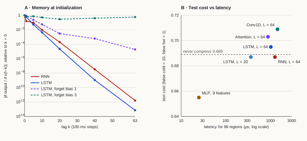
• The decay is geometric. For the RNN, we lose roughly a factor of 10 every 5 to 10 steps: at 63 steps, $10^{-12}$ is left. Panel A of the figure plots these curves on a log scale: they’re roughly straight lines, the signature of a product of similar factors.
• A fresh LSTM is no better off. With $f \approx 0.5$ , its cell forgets as fast as the RNN, even faster beyond 20 steps. The gates only help once they’ve been learned.
• The forget bias changes everything. At 1, we gain about eight orders of magnitude at 63 steps; at 3 ( $f \approx \sigma(3) = 0.95$ ), sensitivity barely decreases at all: the network sees the whole window from the start.

Part 22’s recipe, with an equal budget

For an honest comparison, every model gets exactly the same treatment: AdamW, one-cycle over 20 epochs, clip_grad_norm_ at 1, best epoch on validation, threshold chosen on validation with part 15’s cost. We start with the range test, with two seeds.

# 3. Part 22's recipe for every model: range test, one-cycle, clipping, best epoch
def predict(model, X, batch=8192):
    """Probabilities in batches, in eval() mode and without a graph (memory stays reasonable)."""
    model.eval()
    with torch.no_grad():
        return np.concatenate([torch.sigmoid(model(X[i:i + batch]).squeeze(-1)).numpy()
                               for i in range(0, len(X), batch)])


def lr_range_test(make, X, y, lr_min=1e-5, lr_max=1e3, clip=1.0, seed=0):
    """Part 22's test, for any model: one epoch, step size multiplied at every batch."""
    torch.manual_seed(seed)
    model = make()
    opt = torch.optim.AdamW(model.parameters(), lr=lr_min, weight_decay=1e-4)
    loader = DataLoader(TensorDataset(X, y), batch_size=512, shuffle=True)
    factor = (lr_max / lr_min) ** (1 / (len(loader) - 1))
    loss_fn, lrs, losses, smooth = nn.BCEWithLogitsLoss(), [], [], 0.0
    for i, (xb, yb) in enumerate(loader):
        for g in opt.param_groups:
            g["lr"] = lr_min * factor ** i
        opt.zero_grad()
        loss = loss_fn(model(xb).squeeze(-1), yb)
        loss.backward()
        nn.utils.clip_grad_norm_(model.parameters(), clip)
        opt.step()
        smooth = 0.9 * smooth + 0.1 * loss.item()
        lrs.append(lr_min * factor ** i)
        losses.append(smooth / (1 - 0.9 ** (i + 1)))
        if not np.isfinite(losses[-1]) or losses[-1] > 4 * min(losses):
            break
    return lrs[int(np.argmin(losses))]


def train_model(make, Xtr, ytr, Xva, yva, lr_max, epochs=20, clip=1.0, seed=0):
    """fit (part 22) with one-cycle, plus clip_grad_norm_ between backward() and step()."""
    torch.manual_seed(seed)
    model = make()
    opt = torch.optim.AdamW(model.parameters(), lr=lr_max, weight_decay=1e-4)
    loader = DataLoader(TensorDataset(Xtr, ytr), batch_size=512, shuffle=True)
    scheduler = torch.optim.lr_scheduler.OneCycleLR(opt, max_lr=lr_max, epochs=epochs,
                                                   steps_per_epoch=len(loader))
    loss_fn = nn.BCEWithLogitsLoss()
    best, state, hist = np.inf, None, []
    for epoch in range(1, epochs + 1):
        model.train()
        for xb, yb in loader:
            opt.zero_grad()
            loss_fn(model(xb).squeeze(-1), yb).backward()
            if clip is not None:
                nn.utils.clip_grad_norm_(model.parameters(), clip)   # the total gradient norm <= clip
            opt.step()
            scheduler.step()
        ll_va = log_loss(yva.numpy(), predict(model, Xva), labels=[0, 1])
        hist.append(ll_va)
        if ll_va < best:
            best, state = ll_va, {k: v.clone() for k, v in model.state_dict().items()}
    model.load_state_dict(state)
    return model, hist


def average_cost(y, p, threshold, c_fn=10, c_fp=1):
    return (c_fn * np.sum((y == 1) & (p < threshold)) + c_fp * np.sum((y == 0) & (p >= threshold))) / len(y)


def latency(model, X, n=200):
    """Median time to score 96 regions at once (one aggregation of the trace), in µs."""
    model.eval()
    with torch.no_grad():
        timings = []
        for _ in range(n):
            t0 = time.perf_counter()
            model(X[:96])
            timings.append(time.perf_counter() - t0)
    return 1e6 * np.median(timings)


candidates = {
    "MLP, 9 features":    (lambda: mlp([9, 32, 32, 1]), (Xtr, Xva, Xte)),
    "RNN, L = 64":        (lambda: Recurrent("rnn"), S[64]),
    "LSTM, L = 20":       (lambda: Recurrent("lstm"), S[20]),
    "LSTM, L = 64":       (lambda: Recurrent("lstm"), S[64]),
    "Conv1D, L = 64":     (lambda: Conv1D(), S[64]),
    "Attention, L = 64":  (lambda: Attention(), S[64]),
}
# (a) The range test, with two seeds: it locates the useful zone, but does not settle a factor of 3
for name, (make, (A_tr, _, _)) in candidates.items():
    print(f"{name:>18} | range-test minimum, seeds 0 and 1: "
          + " and ".join(f"{lr_range_test(make, A_tr, ytr, seed=g):.2g}" for g in (0, 1)))

# (b) Equal budget: three max step sizes per model, chosen on validation log-loss, then the test once
thresholds = np.linspace(0.01, 0.99, 99)
y_va, y_te = va.y.to_numpy(), te.y.to_numpy()
print(f"never compress: test cost {average_cost(y_te, np.ones(len(te)), 0.5):.3f}")
models, probas = {}, {}
for name, (make, (A_tr, A_va, A_te)) in candidates.items():
    trials = {}
    for lr_max in (1e-3, 3e-3, 1e-2):
        t0 = time.perf_counter()
        trials[lr_max] = train_model(make, A_tr, ytr, A_va, yva, lr_max) + (time.perf_counter() - t0,)
    lr_max = min(trials, key=lambda k: min(trials[k][1]))
    model, hist, duration = trials[lr_max]
    p_va, p_te = predict(model, A_va), predict(model, A_te)
    s = thresholds[np.argmin([average_cost(y_va, p_va, s) for s in thresholds])]
    models[name], probas[name] = model, (p_va, p_te)
    print(f"{name:>18} | {n_params(model):>5} param. | val by step size: "
          + " / ".join(f"{min(e[1]):.4f}" for e in trials.values())
          + f" | chosen step {lr_max:g} | {duration:3.0f} s | best ep. {int(np.argmin(hist)) + 1:>2} | "
          f"log-loss val {min(hist):.4f} | AUC val {roc_auc_score(y_va, p_va):.3f} | "
          f"AUC test {roc_auc_score(y_te, p_te):.3f} | threshold {s:.2f} | test cost {average_cost(y_te, p_te, s):.3f} | "
          f"{latency(model, A_te):.0f} µs / 96 regions")

The range test first:

Model	Minimum, seed 0	Minimum, seed 1
MLP, 9 features	0.12	0.44
RNN, $L = 64$	0.024	0.077
LSTM, $L = 20$	0.44	0.41
LSTM, $L = 64$	0.066	0.096
Conv1D, $L = 64$	0.1	0.061
Attention, $L = 64$	0.021	0.028

The same model gives a minimum up to 3.7 times different from one seed to the other (MLP: 0.12 vs 0.44). The range test is a good tool to locate the useful zone (here between $10^{-3}$ and a few $10^{-2}$ for all of them), not to settle a factor of 3. Hence the second part of the block: three max step sizes, $10^{-3}$ , $3 \times 10^{-3}$ and $10^{-2}$ , for each model, keeping the best on validation. Six models, eighteen training runs, the same budget for all.

Model	Parameters	Chosen step	Training	Val log-loss	Val AUC	Test AUC	Threshold (val)	Test cost	Latency, 96 regions
MLP, 9 features (part 22)	1,409	$10^{-2}$	17 s	0.2772	0.916	0.873	0.11	0.655	25 µs
RNN, $L = 64$	1,185	$10^{-2}$	100 s	0.3920	0.854	0.823	0.09	0.687	1,265 µs
LSTM, $L = 20$	4,641	$10^{-2}$	48 s	0.4003	0.835	0.793	0.05	0.687	366 µs
LSTM, $L = 64$	4,641	$10^{-2}$	110 s	0.2751	0.911	0.867	0.11	0.695	1,024 µs
Conv1D, $L = 64$	12,673	$3 \times 10^{-3}$	106 s	0.2734	0.913	0.855	0.09	0.709	1,445 µs
Attention, $L = 64$	8,481	$10^{-2}$	109 s	0.3961	0.851	0.817	0.07	0.703	884 µs
Never compress								0.689

• Window length decides everything. The same LSTM goes from a validation AUC of 0.835 with $L = 20$ to 0.911 with $L = 64$ . Periodic regions have periods of 15 to 60 aggregations: a window of 20 often contains nothing but zeros, and the model doesn’t know where it is in the cycle. The 9 features, on the other hand, look back up to 100 (mean_100) and 500 (since_last) time steps.
• The RNN confirms section 2. With the same 64-step window as the LSTM, it stays at 0.854: it can only exploit the end of the window.
• On validation, LSTM and Conv1D match the MLP, and even beat it slightly in log-loss (0.2751 and 0.2734 vs 0.2772). From raw accesses alone, they relearned what the 9 features summarized. That’s already a result: those features were well chosen. (The MLP gets 0.2772 here vs 0.2759 in part 22: clipping and the order of random draws differ, a gap the size of seed-to-seed noise. Its test cost, 0.655 vs 0.626, mostly shows how much the cost depends on the threshold, chosen here at 0.11 instead of 0.07.)
• On the test, none of them beats the MLP, and the two best on validation cost more than “never compress” (0.695 and 0.709 vs 0.689). We come back to this in block 4.
• Attention alone, with one head and one layer, disappoints (0.851). To know where you are in a cycle, you need to spot the last start of activity and then count: a single weighted average of past steps isn’t enough for that. Transformers stack several layers for this.
• Latency is 15 to 58 times higher. 25 µs to score 96 regions with the MLP, 366 µs to 1.4 ms for the sequence models, always on CPU and without optimization. For a daemon that decides every 100 ms, 1 ms is still acceptable; for millions of pages, it’s another matter (part 26, serving a model).
• The best step size is at the edge of the grid for five models out of six ( $10^{-2}$ ). The grid should have gone one notch higher: that’s exercise 5.

What the models learned to look at

# 4. What the models learned to look at
# (a) After training: sensitivity of the output to the input from k steps ago, RNN vs LSTM
xb = S[64][0][:2048].clone().requires_grad_()
for name in ["RNN, L = 64", "LSTM, L = 64"]:
    xb.grad = None
    m = models[name]
    m.eval()
    m(xb).sum().backward()
    g = xb.grad.norm(dim=(0, 2))
    print(f"{name:>13} trained | relative to k = 0: "
          + " ".join(f"k={k}: {(g[-1 - k] / g[-1]).item():.1e}" for k in (1, 5, 10, 20, 40, 63)))

# (b) Where does attention look? Mean weights by lag, on validation
att = models["Attention, L = 64"]
att.eval()
with torch.no_grad():
    att(S[64][1][:8192])
weights = att.weights[:, 0].mean(0).numpy()[::-1]          # weights[k]: lag k (0 = time t)
print("attention: mean weight of lags 0..4:", np.round(weights[:5], 3),
      "| mass on the last 10 steps:", round(float(weights[:10].sum()), 3),
      "| most attended lags:", np.argsort(weights)[::-1][:5])

# (c) Before and after the regime change at t = 2100: where each model wins or loses
before = (te.t < 2100).to_numpy()
for name, (p_va, p_te) in probas.items():
    s = thresholds[np.argmin([average_cost(y_va, p_va, s) for s in thresholds])]
    print(f"{name:>18} | test AUC before 2100 {roc_auc_score(y_te[before], p_te[before]):.3f}, "
          f"after {roc_auc_score(y_te[~before], p_te[~before]):.3f} | cost before {average_cost(y_te[before], p_te[before], s):.3f}, "
          f"after {average_cost(y_te[~before], p_te[~before], s):.3f}")
print(f"never compress | cost before {average_cost(y_te[before], np.ones(before.sum()), 0.5):.3f}, "
      f"after {average_cost(y_te[~before], np.ones((~before).sum()), 0.5):.3f}")

Memory after training. Same measurement as in block 2, over 2,048 windows, with the trained models:

Trained model	$k = 1$	$k = 5$	$k = 10$	$k = 20$	$k = 40$	$k = 63$
RNN, $L = 64$	0.95	0.14	$1.0 \times 10^{-2}$	$5.5 \times 10^{-5}$	$1.2 \times 10^{-9}$	$1.1 \times 10^{-10}$
LSTM, $L = 64$	0.24	$4.3 \times 10^{-2}$	$3.7 \times 10^{-2}$	$2.0 \times 10^{-2}$	$4.5 \times 10^{-3}$	$5.9 \times 10^{-2}$

Training changed nothing for the RNN: beyond 20 steps, the window is invisible. The LSTM, on the other hand, learned to keep its forget gates open: the sensitivity to the input from 63 steps ago (0.059) is of the same order as from 5 steps ago. It learned to use the whole window, even though it started from the same point as the RNN.

Where attention looks. On average over 8,192 validation windows, the weight of the present step is practically zero (less than 0.001): the head already receives time $t$ directly, it doesn’t need to listen to it. The last 10 steps get 28.5% of the weight, and the most attended lags are 27, 38, 28, 7 and 29 steps back, within the range of simulated periods. Readable, but not enough to predict well.

Before and after the regime change. The test starts at $t = 1800$ and contains the workload change at $t = 2100$ (part 14). We separate the two periods:

Model	Test AUC before 2100	Test AUC after	Cost before	Cost after
MLP, 9 features	0.896	0.865	0.605	0.671
RNN, $L = 64$	0.838	0.818	0.674	0.692
LSTM, $L = 20$	0.826	0.782	0.649	0.699
LSTM, $L = 64$	0.896	0.857	0.633	0.716
Conv1D, $L = 64$	0.897	0.839	0.607	0.743
Attention, $L = 64$	0.842	0.809	0.673	0.712
Never compress			0.697	0.686

This is the real lesson of the article. Before the change, Conv1D and LSTM do exactly as well as the MLP (AUC 0.897 and 0.896 vs 0.896). After, they lose more: 0.839 and 0.857 vs 0.865, and their cost goes above “never compress”. The 9 features are relative, generic quantities (time since the last access, estimated period) that keep their meaning when a region changes nature. The filters and gates learned on raw accesses fit the pre-change patterns more tightly. More capacity, more dependence on the training regime.

---

Running project: what this changes for the thesis

• H2 now has a protocol. Same split, same purge, same recipe (one-cycle, clipping, best epoch), same step-size grid for every model, threshold chosen on validation, part 15’s cost. The LSTM is H2’s upper reference; on this simulation, it is not above the MLP on features. That’s a publishable result as is, provided you show it before and after a regime change.
• The window is a first-order hyperparameter. $L$ must cover the longest expected periods. On real DAMON traces (100 ms aggregations, JVM GC cycles of several seconds), that can mean $L$ of several hundred, hence slower LSTMs, or a more dilated Conv1D.
• Features aren’t a crutch. On validation, LSTM and Conv1D relearned the 9 features from raw accesses; on the test, the features generalize better. The Discussion chapter can put it this way: a sequence model’s gain must come from patterns the features don’t capture, and real traces are the place to look for them (irregular accesses, interactions between regions).
• The hybrid model is the natural candidate: an LSTM on the raw window whose final state is concatenated with the 9 features before the head. That’s exercise 3.
• Latency goes into the results table. 25 µs vs about 1 ms for 96 regions: to be measured on the target machine, with the same protocol (median over 200 calls), in the Experiments chapter.

---

Hands-on exercise

1. LSTM or GRU? Replace Recurrent("lstm") with Recurrent("gru") with $L = 64$ and a max step size of $10^{-2}$ . Compare the number of parameters, validation log-loss, test AUC and cost, training time and latency.
2. The forget bias, once trained. Block 2 showed that a forget bias of 3 keeps the whole window visible at initialization. Train Recurrent("lstm", forget_bias=3.0) with $L = 64$ (max step size $10^{-2}$ ). Does that initial memory gain translate into performance at the end?
3. The hybrid model. Write a module that feeds the window’s 2 channels into an LSTM, concatenates its last hidden state (32 values) with the row’s 9 standardized features, then applies a Linear(41, 32) → ReLU → Linear(32, 1) head. Tip: to reuse train_model without changing it, paste the 9 features at every step of the window (an (n, 64, 11) tensor) and split them apart in forward. Compare with the MLP and the LSTM alone, before and after $t = 2100$ .
4. A longer window. Redo the LSTM with $L = 100$ (the window of mean_100). Note the training time and latency: are they proportional to $L$ ?
5. Extending the grid. For five models out of six, the best step size was the largest in the grid. Add $3 \times 10^{-2}$ and see whether the ranking changes.
6. Running project. Write H2’s protocol for the Methodology chapter (models, window, step-size grid, number of epochs, seeds, metrics, latency), then measure on a real DAMON trace the longest access period you observe. What value of $L$ do you deduce?

Hints. Question 1: the GRU has 3,489 parameters, 25% fewer than the LSTM in the recurrent part. Best epoch 12, validation log-loss 0.2725, validation AUC 0.911, test AUC 0.871, threshold 0.03, test cost 0.623: the best cost in the article, but with a threshold so low that a slight calibration shift would tip it over, to be confirmed over several seeds. Training 193 s and latency 2,918 µs: on this CPU, the GRU implementation is slower than the LSTM’s despite less computation. Always measure latency, don’t infer it from the number of parameters. Question 2: best epoch 8, validation log-loss 0.2769, validation AUC 0.913, test AUC 0.863, cost 0.682: no better than the default LSTM (0.2751). With 123,840 windows and 20 epochs, the LSTM learns on its own to open its gates (block 4); the forget bias matters mostly for longer windows or scarcer data. Question 3: 5,985 parameters, best epoch 17, validation log-loss 0.2642 (the best in the article), validation AUC 0.913, test AUC 0.862 (0.892 before 2100, 0.850 after), threshold 0.04, cost 0.629. The hybrid is the best calibrated on validation, but it too loses more than the MLP after the regime change: the sequence part adds dependence on the training regime.

---

Further resources

• Christopher Olah, Understanding LSTM Networks (2015): the diagrams that make the gates obvious.
• Hochreiter & Schmidhuber, Long Short-Term Memory (Neural Computation, 1997); Pascanu, Mikolov & Bengio, On the difficulty of training recurrent neural networks (ICML 2013): vanishing and exploding gradients, and clipping.
• Jozefowicz, Zaremba & Sutskever, An Empirical Exploration of Recurrent Network Architectures (ICML 2015): the forget bias at 1, and GRU vs LSTM.
• Bai, Kolter & Koltun, An Empirical Evaluation of Generic Convolutional and Recurrent Networks for Sequence Modeling (2018): dilated convolutions (TCN) against LSTMs.
• Vaswani et al., Attention Is All You Need (NeurIPS 2017): queries, keys, values and the $1/\sqrt{d}$ factor.
• Hashemi et al., Learning Memory Access Patterns (ICML 2018): LSTMs to predict memory accesses, the work closest to your thesis.
• Dive into Deep Learning, chapters Recurrent Neural Networks and Attention Mechanisms.
• Refreshers: M1 · Vectors and dot product, M5 · Chain rule, part 22 · Training a neural network well.

---

What you should be able to do before moving on

• Turn a trace into (batch, L, channels) windows without leakage: a window that stops at $t$ , train-only statistics
• Explain with the chain rule why an RNN forgets geometrically, and measure that memory with $\partial \text{output} / \partial x_{t-k}$
• Write an LSTM in PyTorch, and initialize its forget bias
• Compute the receptive field of a dilated Conv1D
• Write an attention head, and read its weights
• Compare a sequence model with a feature-based model at equal budget, before and after a regime change, latency included
• Choose $L$ based on the periods the model needs to see

Next part: Running project: is this page hot or cold? (part 24). We put everything together into a complete, reproducible project, against the LRU and CLOCK baselines and Belady’s oracle, with several seeds, and we plot the “false colds vs inference cost” Pareto front where this article’s LSTM will take its place.