November 1, 2026 · 26 min read

Training a neural network well

Learning-rate range test, SGD, momentum and Adam, initialization, LayerNorm, dropout and weight decay: we break an MLP's training on purpose, read the curves, then fix it.

Mastering AI · Technical phase · Week 3 · Part 22

Goal of this step

In part 21, we wrote a PyTorch training loop that works, with the default settings: AdamW, a step size of $10^{-3}$ , 20 epochs. The network never overfit, and we never had to wonder whether the step size was right. That comfort won’t last: the sequence models of part 23 are deeper, slower to train, and much more sensitive to these settings.

This article is a diagnostic toolbox. We’ll deliberately break training in several ways, look at what each failure looks like on the curves, then fix it.

By the end of this article you’ll be able to:

pick a starting learning rate with a learning-rate range test instead of guessing it;
compare SGD, momentum and Adam and explain their differences with the maths of M10;
explain why initialization decides whether a deep network learns, and what normalization fixes;
trigger overfitting, then fight it with early stopping, weight decay and dropout;
read a loss curve: divergence, plateau, overfitting, underfitting.

Key concepts

1. The learning rate, the setting that matters most

Intuition. You’re walking down a valley in the fog. With ant-sized steps, you never reach the bottom. With giant steps, you jump over the bottom and land on the other slope, higher and higher. In between, there’s a range of step sizes where you go down fast without oscillating.

In M6, we saw that on a quadratic, gradient descent only converges if $\eta < 2/\lambda_{\max}$ , where $\lambda_{\max}$ is the largest curvature. On a network, we don’t know $\lambda_{\max}$ , and it changes during training. Hence an empirical method, the learning-rate range test (Leslie Smith, 2017):

start from a tiny step size ( $10^{-5}$ );
at each mini-batch, multiply it by a constant factor, so as to reach a huge step size ( $10^{3}$ ) within a single epoch;
plot the (smoothed) loss against the step size, on a log scale.

The loss doesn’t move while the step is too small, then goes down, then explodes. We pick a step size about ten times smaller than the one at the minimum: large enough to make progress, with a margin before instability.

2. SGD, momentum, Adam: three ways to take a step

Intuition. SGD follows the current slope. Momentum adds inertia: a rolling ball builds up speed in consistent directions and damps the zigzags. Adam additionally gives each parameter its own step size.

\begin{aligned} \text{SGD:}\quad & \theta \leftarrow \theta - \eta\, g \\ \text{momentum:}\quad & v \leftarrow \beta v + g, \qquad \theta \leftarrow \theta - \eta\, v \\ \text{Adam:}\quad & \theta \leftarrow \theta - \eta\, \frac{\hat m}{\sqrt{\hat v} + \varepsilon} \end{aligned}

Two direct consequences, which we’ll check in the code:

with momentum $\beta = 0.9$ , a constant gradient produces a velocity $g/(1 - \beta) = 10\,g$ : the effective step is ten times larger. SGD with momentum and $\eta = 0.01$ should therefore behave roughly like SGD without momentum and $\eta = 0.1$ ;
Adam divides the mean gradient $\hat m$ by its own magnitude $\sqrt{\hat v}$ . Each parameter therefore moves by about $\eta$ per step, whatever the size of its gradient, as long as it is clearly above $\varepsilon = 10^{-8}$ . That’s very convenient (fewer settings), but it can also hide a problem, as we’ll see with initialization.

AdamW is Adam with decoupled weight decay: at each step, $\theta \leftarrow \theta - \eta \lambda \theta$ , applied separately, instead of adding $\lambda \lVert \theta \rVert^2$ to the loss. It’s the L2 penalty of M11, written so that Adam doesn’t renormalize it.

3. Initialization: keeping the signal at the right size

Intuition. A deep network is a chain of multiplications. If each layer multiplies the size of the signal by 0.5, after 16 layers only $0.5^{16} \approx 1.5 \times 10^{-5}$ of the signal remains. By 2, it gets multiplied by 65,536. The gradient, which travels back up the same chain (M5), suffers the same fate: it vanishes or it explodes.

With the variances of M7, for a layer with $n_{\text{in}}$ inputs, independent weights of variance $\operatorname{Var}(w)$ and a ReLU (which zeroes half of the signal):

\operatorname{Var}(z_{\ell+1}) \approx \frac{n_{\text{in}} \operatorname{Var}(w)}{2} \, \operatorname{Var}(z_\ell)

For the signal to keep its size, this factor must equal 1, i.e. $\operatorname{Var}(w) = 2 / n_{\text{in}}$ : that’s He initialization (2015), designed for ReLU. Xavier initialization (Glorot, 2010), $\operatorname{Var}(w) = 2/(n_{\text{in}} + n_{\text{out}})$ , was designed for symmetric activations like tanh; with a ReLU and layers of 64, it gives a factor of $1/2$ in variance, i.e. about 0.7 in standard deviation per layer. The default initialization of nn.Linear gives $\operatorname{Var}(w) = 1/(3 n_{\text{in}})$ , a factor of about 0.4 per layer: fine for 2 layers, not for 16.

4. Normalization: rescaling the signal at every layer

Intuition. Rather than relying on a perfect initialization, we bring the signal back to mean 0 and variance 1 at every layer, then let the network choose the scale it wants.

\operatorname{LN}(z) = \gamma \odot \frac{z - \mu}{\sqrt{\sigma^2 + \varepsilon}} + \beta

LayerNorm computes $\mu$ and $\sigma$ over the neurons of a single example. It behaves the same in training and in production, whatever the batch size. It’s the normalization of LSTMs and Transformers (part 23).
BatchNorm computes $\mu$ and $\sigma$ over the examples of the mini-batch, and keeps running averages for evaluation. That’s why model.eval() changes its behavior (part 21). It dominates in vision; we don’t use it here.

5. Regularizing: early stopping, weight decay, dropout

Intuition. A network large enough to learn the noise will end up learning it. Three brakes, from the simplest to the subtlest:

Technique	What it does	Link with the maths
Early stopping	stop when validation hasn’t improved for `patience` epochs, and keep the best epoch	limiting the number of steps limits how far we move from the initialization, an effect close to L2
Weight decay	every weight is pulled towards 0 at every step	the L2 penalty of M11, the constraint $\lVert \theta \rVert \le r$
Dropout	during training, each neuron is switched off with probability $p$ , survivors are multiplied by $1/(1-p)$ ; at evaluation, nothing is switched off	the network can no longer rely on one specific neuron: it’s an average over many sub-networks

6. Changing the step size during training

Intuition. At the start, we want big steps to cross the landscape; at the end, small steps to settle at the bottom without bouncing. A scheduler changes $\eta$ over the iterations. The one-cycle policy (Smith, 2018) first raises the step from $\eta_{\max}/25$ to $\eta_{\max}$ over 30% of the iterations, then brings it back down along a cosine to almost 0. We take $\eta_{\max}$ from the range given by the range test.

Code example

As in parts 15 to 21, we reuse the part 14 script as is (simulation and dataset), then append the five blocks below. We reuse the split of part 15 and the inputs of part 21 (log1p then standardization with train-only statistics). The whole thing runs in about four minutes on a two-core CPU (numpy 2.5, pandas 3.0, scikit-learn 1.9, torch 2.14).

The tools, and the learning-rate range test

The fit function is part 21’s loop, with three additions: an optional step-size scheduler, stopping if the loss becomes infinite, and early stopping. It always keeps the best epoch on validation.

import time
import torch
from torch import nn
from torch.utils.data import TensorDataset, DataLoader
from sklearn.metrics import log_loss

torch.set_num_threads(2)

# Part 15's split: train t < 1390, validation 1400 <= t < 1790, test t >= 1800
tr = df[df.t < 1390]
va = df[(df.t >= 1400) & (df.t < 1790)]
te = df[df.t >= 1800]


def tensors(d):
    """log1p, then standardization with train statistics only (part 21)."""
    A, R = np.log1p(d[FEATURES]), np.log1p(tr[FEATURES])
    A = (A - R.mean()) / R.std()
    return (torch.tensor(A.to_numpy(), dtype=torch.float32),
            torch.tensor(d.y.to_numpy(), dtype=torch.float32))


Xtr, ytr = tensors(tr)
Xva, yva = tensors(va)
Xte, yte = tensors(te)


def mlp(widths, p_dropout=0.0, norm=False):
    """widths = [9, 32, 32, 1] -> Linear/ReLU stack; optional LayerNorm and Dropout after each hidden layer."""
    layers = []
    for a, b in zip(widths[:-2], widths[1:-1]):
        layers += [nn.Linear(a, b)] + ([nn.LayerNorm(b)] if norm else []) + [nn.ReLU()]
        layers += [nn.Dropout(p_dropout)] if p_dropout > 0 else []
    layers.append(nn.Linear(widths[-2], widths[-1]))
    return nn.Sequential(*layers)


def evaluate(model, X, y):
    model.eval()
    with torch.no_grad():
        p = torch.sigmoid(model(X).squeeze(-1)).numpy()
    return roc_auc_score(y.numpy(), p), log_loss(y.numpy(), p, labels=[0, 1])


def fit(model, opt, Xtr, ytr, Xva, yva, epochs=20, batch=512, scheduler=None, patience=None, seed=0):
    """Part 21's loop + three additions: per-step scheduler, divergence detection, early stopping."""
    torch.manual_seed(seed)
    loss_fn = nn.BCEWithLogitsLoss()
    loader = DataLoader(TensorDataset(Xtr, ytr), batch_size=batch, shuffle=True)
    best, state, hist, waited = np.inf, None, [], 0
    for epoch in range(1, epochs + 1):
        model.train()
        total = 0.0
        for xb, yb in loader:
            opt.zero_grad()
            loss = loss_fn(model(xb).squeeze(-1), yb)
            loss.backward()
            opt.step()
            if scheduler is not None:
                scheduler.step()                  # one-cycle: the step size changes at every batch
            total += loss.item() * len(yb)
        if not np.isfinite(total):                # divergence: the loss became inf or nan
            hist.append((epoch, np.nan, np.nan, np.nan))
            break
        auc_va, ll_va = evaluate(model, Xva, yva)
        hist.append((epoch, total / len(ytr), ll_va, auc_va))
        if ll_va < best:
            best, state, waited = ll_va, {k: v.clone() for k, v in model.state_dict().items()}, 0
        else:
            waited += 1
            if patience is not None and waited >= patience:
                break                             # early stopping
    if state is not None:
        model.load_state_dict(state)              # we keep the best epoch on validation
    return hist


# 1. Learning-rate range test (Smith, 2017): a single epoch, step size multiplied at every batch
def lr_range_test(make_opt, lr_min=1e-5, lr_max=1e3, seed=0):
    torch.manual_seed(seed)
    model = mlp([9, 32, 32, 1])
    opt = make_opt(model.parameters(), lr_min)
    loader = DataLoader(TensorDataset(Xtr, ytr), batch_size=512, shuffle=True)
    factor = (lr_max / lr_min) ** (1 / (len(loader) - 1))
    loss_fn, lrs, losses, smooth = nn.BCEWithLogitsLoss(), [], [], 0.0
    for i, (xb, yb) in enumerate(loader):
        lr = lr_min * factor ** i
        for g in opt.param_groups:
            g["lr"] = lr
        opt.zero_grad()
        loss = loss_fn(model(xb).squeeze(-1), yb)
        loss.backward()
        opt.step()
        smooth = 0.9 * smooth + 0.1 * loss.item()             # exponential moving average...
        lrs.append(lr)
        losses.append(smooth / (1 - 0.9 ** (i + 1)))          # ...with bias correction (like Adam)
        if not np.isfinite(losses[-1]) or losses[-1] > 4 * min(losses):
            break                                             # the loss explodes: stop
    i_min = int(np.argmin(losses))
    return lrs, losses, lrs[i_min], lrs[-1]


for name, make_opt in [("AdamW", lambda p, lr: torch.optim.AdamW(p, lr=lr, weight_decay=1e-4)),
                       ("SGD momentum 0.9", lambda p, lr: torch.optim.SGD(p, lr=lr, momentum=0.9))]:
    lrs, losses, lr_best, lr_stop = lr_range_test(make_opt)
    print(f"{name:>16} | min smoothed loss {min(losses):.3f} at lr = {lr_best:.2g} | "
          f"explodes at lr = {lr_stop:.2g} | suggested lr ~ {lr_best / 10:.1g}")

Output:

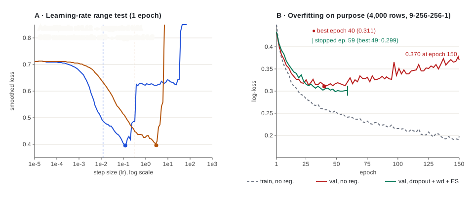
           AdamW | min smoothed loss 0.396 at lr = 0.12 | explodes at lr = 69 | suggested lr ~ 0.01
SGD momentum 0.9 | min smoothed loss 0.396 at lr = 3 | explodes at lr = 7 | suggested lr ~ 0.3

Panel A of the figure shows both curves. For AdamW, the loss starts going down around $10^{-3}$ , reaches its minimum at 0.12, then jumps back up to about 0.62 and stays there before exploding. The suggested step is therefore $10^{-2}$ , ten times the default $10^{-3}$ . For SGD with momentum, the whole curve is shifted right by a factor of about 25: the minimum is at 3, the suggested step at 0.3. The same “lr” number means something completely different from one optimizer to another.

Three optimizers, twelve settings, one grid

We check these predictions by training the same 9-32-32-1 MLP, with the same seed, for 8 epochs per setting.

# 2. The same MLP, three optimizers, several step sizes, 8 epochs each
configs = [("SGD", 0.01), ("SGD", 0.1), ("SGD", 1.0),
           ("SGD momentum", 0.01), ("SGD momentum", 0.1), ("SGD momentum", 1.0), ("SGD momentum", 10.0),
           ("AdamW", 1e-4), ("AdamW", 1e-3), ("AdamW", 1e-2), ("AdamW", 1e-1), ("AdamW", 1.0)]
base_rate = yva.mean().item()
print(f"reference: always predicting the base rate {base_rate:.3f} gives a val log-loss of "
      f"{log_loss(yva.numpy(), np.full(len(yva), base_rate)):.4f}")
curves = {}
for opt_name, lr in configs:
    torch.manual_seed(0)
    model = mlp([9, 32, 32, 1])
    if opt_name == "AdamW":
        opt = torch.optim.AdamW(model.parameters(), lr=lr, weight_decay=1e-4)
    else:
        opt = torch.optim.SGD(model.parameters(), lr=lr, momentum=0.9 if "momentum" in opt_name else 0.0)
    t0 = time.perf_counter()
    hist = fit(model, opt, Xtr, ytr, Xva, yva, epochs=8)
    curves[(opt_name, lr)] = hist
    val = [h[2] for h in hist]
    print(f"{opt_name:>12} lr={lr:<6g} | val log-loss ep. 1 {val[0]:.4f} -> ep. {len(val)} {val[-1]:.4f} | "
          f"best {np.nanmin(val):.4f} | train {hist[-1][1]:.4f} | {time.perf_counter() - t0:.0f} s")

The reference first: always predicting the validation base rate (0.301) gives a log-loss of 0.6116. Remember that number; it comes back.

Optimizer	Step size	Val log-loss, epoch 1	Epoch 8	Best
SGD	0.01	0.5624	0.4464	0.4464
SGD	0.1	0.4368	0.3314	0.3314
SGD	1	0.3514	0.2884	0.2884
SGD momentum	0.01	0.4404	0.3331	0.3331
SGD momentum	0.1	0.3344	0.2939	0.2895
SGD momentum	1	0.3027	0.2874	0.2856
SGD momentum	10	0.6949	0.6524	0.6116
AdamW	0.0001	0.6003	0.4154	0.4154
AdamW	0.001	0.4107	0.2978	0.2978
AdamW	0.01	0.3107	0.2869	0.2832
AdamW	0.1	0.3000	0.2853	0.2853
AdamW	1	0.6118	0.6116	0.6116

Momentum does multiply the step by ten. SGD with momentum at 0.01 (0.3331) does almost exactly what SGD without momentum does at 0.1 (0.3314). That’s the $g/(1-\beta)$ formula of section 2.
The range test was right. The best AdamW is at $10^{-2}$ (0.2832), the step it suggested. With the default $10^{-3}$ , after 8 epochs we’re still at 0.2978: the default isn’t wrong, it’s slow.
Too small is slow; too large is broken. AdamW at $10^{-4}$ and SGD at 0.01 are still going down at epoch 8. Those are underfitting plateaus, not minima.
Here, divergence doesn’t produce nan: it produces a constant. SGD with momentum at 10 and AdamW at 1 end at 0.6116, exactly the log-loss of “always predict 0.301”. In both cases (we checked afterwards), a step that was too large pushed the 32 ReLUs of the second hidden layer into the negative zone for every input: they output 0, their gradient is zero, and they’ll never wake up. Only the output bias still learns, and it learns the base rate. That’s the failure we reproduce in exercise 1.

Initialization and normalization in a deep network

To see gradients vanish, we need depth: we stack 16 hidden layers of 64 ReLUs. For each initialization, we measure the size of the signal at the last hidden layer and the gradient norm of the first and sixteenth layers, on a batch of 512 rows, before any training. Then we train for 3 epochs with AdamW.

# 3. Initialization and gradient flow in a deep network: 16 hidden layers of 64 ReLUs
def deep_net(init, norm=False, depth=16, width=64):
    torch.manual_seed(0)
    model = mlp([9] + [width] * depth + [1], norm=norm)
    for m in model:
        if isinstance(m, nn.Linear):
            nn.init.zeros_(m.bias)
            if init == "N(0, 0.01)":
                nn.init.normal_(m.weight, std=0.01)
            elif init == "Xavier":
                nn.init.xavier_normal_(m.weight)          # Var(w) = 2 / (n_in + n_out)
            elif init == "He":
                nn.init.kaiming_normal_(m.weight, nonlinearity="relu")   # Var(w) = 2 / n_in
    return model


xb, yb = Xtr[:512], ytr[:512]
for init, norm in [("N(0, 0.01)", False), ("Xavier", False), ("He", False), ("PyTorch default", False),
                   ("PyTorch default", True)]:
    model = deep_net(init, norm)
    linears = [m for m in model if isinstance(m, nn.Linear)]
    h = xb
    for m in model[:-1]:
        h = m(h)
    nn.BCEWithLogitsLoss()(model(xb).squeeze(-1), yb).backward()
    g_first, g_last = linears[0].weight.grad.norm().item(), linears[-2].weight.grad.norm().item()
    hist = fit(model, torch.optim.AdamW(model.parameters(), lr=1e-3, weight_decay=1e-4),
               Xtr, ytr, Xva, yva, epochs=3)
    label = init + (" + LayerNorm" if norm else "")
    print(f"{label:>23} | std of last hidden layer {h.std().item():.1e} | grad. layer 1 {g_first:.1e} "
          f"/ layer 16 {g_last:.1e} | val log-loss after 3 epochs {hist[-1][2]:.4f}")

Initialization	Std, hidden layer 16	Gradient layer 1	Gradient layer 16	Val log-loss after 3 epochs
$\mathcal{N}(0,\, 0.01)$	$2.0 \times 10^{-21}$	$6.9 \times 10^{-21}$	$7.0 \times 10^{-21}$	0.6116
Xavier	$9.4 \times 10^{-4}$	$3.4 \times 10^{-3}$	$4.6 \times 10^{-3}$	0.2916
He	0.48	0.37	1.1	0.2858
PyTorch default	$3.8 \times 10^{-7}$	$2.2 \times 10^{-7}$	$1.7 \times 10^{-6}$	0.2866
PyTorch default + LayerNorm	0.58	0.73	2.3	0.2912

The formula of section 3 checks out. With $\mathcal{N}(0,\, 0.01)$ , each layer multiplies the standard deviation by $\sqrt{64 \times 10^{-4} / 2} \approx 0.057$ : in 16 layers, the signal falls to $10^{-21}$ . With the PyTorch default, the factor is about 0.4 per layer: $3.8 \times 10^{-7}$ at the end. With He, the signal keeps a size of order 1.
Adam rescues almost everything, and that’s misleading. With the PyTorch default, gradients are around $10^{-7}$ , yet the network learns (0.2866): Adam divides by $\sqrt{\hat v}$ , so a gradient of $10^{-7}$ gives the same step as a gradient of 1. With $\mathcal{N}(0,\, 0.01)$ , gradients of $10^{-20}$ are drowned under $\varepsilon = 10^{-8}$ : the step is about $10^{-3} \times 10^{-20} / 10^{-8} \approx 10^{-15}$ , and the network stays at 0.6116, the constant. SGD has no such safety net: that’s exercise 2.
LayerNorm repairs the signal without touching the initialization. With the same default initialization, the signal stays of order 1 (0.58), and so do the gradients. In this network, with Adam, it doesn’t improve the final result (0.2912 vs 0.2866); it matters most when the initialization is bad or the network is recurrent.

Overfitting on purpose, then regularizing

Part 21’s MLP didn’t overfit: 1,409 parameters for 123,840 examples. To study regularization, we first need a network that overfits. We trigger it by flipping the ratio: a 9-256-256-1 network (68,609 parameters) on 4,000 rows drawn at random from the training set, for 150 epochs. Validation and test stay the same.

# 4. Overfitting on purpose: 4,000 training rows, a 9-256-256-1 network, 150 epochs
g = np.random.default_rng(0)
small = torch.tensor(g.choice(len(Xtr), 4000, replace=False))
Xs, ys = Xtr[small], ytr[small]


def regularization(name, wd=0.0, p_dropout=0.0, patience=None, epochs=150):
    torch.manual_seed(0)
    model = mlp([9, 256, 256, 1], p_dropout=p_dropout)
    opt = torch.optim.AdamW(model.parameters(), lr=1e-3, weight_decay=wd)
    hist = fit(model, opt, Xs, ys, Xva, yva, epochs=epochs, batch=128, patience=patience)
    best = min(hist, key=lambda r: r[2])
    print(f"{name:>26} | best ep. {best[0]:>3} / {len(hist):>3} run | train {hist[-1][1]:.4f} | "
          f"val at best {best[2]:.4f}, at the end {hist[-1][2]:.4f} | AUC test {evaluate(model, Xte, yte)[0]:.3f}")
    return hist


n_params = sum(p.numel() for p in mlp([9, 256, 256, 1]).parameters())
print(f"{n_params} parameters for {len(ys)} examples")
over = {
    "no regularization": regularization("no regularization"),
    "early stopping (10)": regularization("early stopping (10)", patience=10),
    "weight decay 0.1": regularization("weight decay 0.1", wd=0.1),
    "dropout 0.3": regularization("dropout 0.3", p_dropout=0.3),
    "dropout 0.3 + wd 0.1 + ES": regularization("dropout 0.3 + wd 0.1 + ES", wd=0.1, p_dropout=0.3, patience=10),
}

Setting (68,609 parameters, 4,000 examples)	Best epoch / run	Train log-loss (end)	Val at best	Val at the end	Test AUC
No regularization	40 / 150	0.1977	0.3106	0.3700	0.859
Early stopping (patience 10)	40 / 50	0.2480	0.3106	0.3190	0.859
Weight decay 0.1	52 / 150	0.2178	0.3083	0.3305	0.862
Dropout 0.3	73 / 150	0.2420	0.2983	0.3117	0.867
Dropout 0.3 + weight decay 0.1 + early stopping	49 / 59	0.2766	0.2991	0.3009	0.868

Panel B of the figure shows the signature of overfitting: the training loss goes down forever (to 0.19), validation reaches its minimum at epoch 40 (0.311), then climbs back up to 0.370.

Early stopping doesn’t change the model; it saves compute. fit always keeps the best epoch: without regularization as with early stopping, we get the same model (0.3106, AUC 0.859). The difference is 50 epochs instead of 150. Without that best-epoch checkpoint, we would have kept the epoch-150 model (0.3700).
Weight decay helps a little; dropout helps most. Weight decay 0.1 shifts the minimum (epoch 52) and lowers it slightly (0.3083). Dropout 0.3 really lowers it (0.2983): the network can no longer memorize by relying on a few specific neurons.
Combined, we almost get back the network trained on everything. With 31 times less data, the combination reaches a test AUC of 0.868, the same as part 21’s MLP trained on all 123,840 rows. All the gain comes from a brake on learning the noise.
The training loss isn’t a goal. The best validation goes with a higher training loss (0.2766 vs 0.1977). A model that fits the training set too well is exactly what we want to avoid.

Back to all the data: one-cycle

We go back to the 123,840 rows and part 21’s 9-32-32-1 network, using the step suggested by the range test as the maximum step of a one-cycle schedule.

# 5. Back to all the data: constant step size (part 21) vs one-cycle
def average_cost(y, p, threshold, c_fn=10, c_fp=1):
    return (c_fn * np.sum((y == 1) & (p < threshold)) + c_fp * np.sum((y == 0) & (p >= threshold))) / len(y)


thresholds = np.linspace(0.01, 0.99, 99)
for name in ["constant lr 1e-3", "one-cycle max 1e-2"]:
    torch.manual_seed(0)
    model = mlp([9, 32, 32, 1])
    opt = torch.optim.AdamW(model.parameters(), lr=1e-3, weight_decay=1e-4)
    sched = None
    if name.startswith("one-cycle"):
        sched = torch.optim.lr_scheduler.OneCycleLR(opt, max_lr=1e-2, epochs=20,
                                                    steps_per_epoch=int(np.ceil(len(ytr) / 512)))
    t0 = time.perf_counter()
    hist = fit(model, opt, Xtr, ytr, Xva, yva, epochs=20, scheduler=sched)
    best = min(hist, key=lambda r: r[2])
    model.eval()
    with torch.no_grad():
        p_va, p_te = (torch.sigmoid(model(X).squeeze(-1)).numpy() for X in (Xva, Xte))
    s = thresholds[np.argmin([average_cost(va.y.to_numpy(), p_va, s) for s in thresholds])]
    print(f"{name:>18} | best ep. {best[0]:>2} | val log-loss {best[2]:.4f} | AUC val {best[3]:.3f} | "
          f"AUC test {roc_auc_score(te.y, p_te):.3f} | threshold {s:.2f} | test cost "
          f"{average_cost(te.y.to_numpy(), p_te, s):.3f} | {time.perf_counter() - t0:.0f} s")

Step size, 20 epochs	Best epoch	Val log-loss	Val AUC	Test AUC	Threshold (val)	Test cost
Constant $10^{-3}$ (part 21)	19	0.2907	0.906	0.869	0.08	0.645
One-cycle, max $10^{-2}$	20	0.2759	0.915	0.872	0.07	0.626
Never compress						0.689

Same network, same number of epochs, better everywhere. One-cycle gains 0.015 of validation log-loss, 0.9 points of validation AUC, and brings the test cost (a false cold costs 10, a false hot 1, as in part 15) down from 0.645 to 0.626, still below “never compress” (0.689).
The constant step doesn’t exactly reproduce part 21 (0.2907 here vs 0.2901): the network is built by mlp instead of the MLP class, and the seed is reset before batch shuffling. The order of random draws changes, the conclusions don’t. It’s also a reminder: a 0.001 difference between two seeds is not a result.
Caution about the test. One seed, one split: as in part 21, the cost gain must be confirmed over several seeds before it is quoted. Exercise 5 varies the maximum step.

Reading a loss curve

This table sums up the failures we met in this article. It’s the first thing to look at when training disappoints.

What you see	Likely diagnosis	First fix
The loss becomes `nan` or `inf`	step far too large, or unstable loss (sigmoid then log instead of `BCEWithLogitsLoss`)	divide the step by 10; loss on logits
The loss freezes at the constant’s value (here 0.6116)	silent divergence: dead ReLUs after a step that was too large, or a gradient drowned at initialization	range test, then a step 10 times smaller; check gradient norms layer by layer
Train and val go down together, slowly, still at the end	step too small, or not enough epochs	range test, one-cycle
Train and val stall together too high	underfitting: network too small or insufficient features	wider network, better features (part 19)
Train goes down, val goes up	overfitting	keep the best epoch, dropout, weight decay, more data
Val swings a lot from one epoch to the next	step too large at the end of training, or validation too small	a schedule that decays the step; more validation data

A method rule, borrowed from Karpathy: before training on everything, check that your network can overfit a tiny sample. If it can’t even memorize 4,000 rows, the problem is in the code (loss, data, step size), not in the regularization.

Running project: what this changes for the thesis

The training protocol becomes a written recipe. For every network in the Experiments chapter (MLP, then LSTM in part 23): range test, step = minimum / 10, one-cycle, best epoch on validation, early stopping. It’s short to write in the Methodology and it heads off the objection “you tuned the LSTM better than the MLP” (or the reverse).
The step size is a hyperparameter like any other. It must be chosen on validation, with the same budget for every compared model, like the number of leaves of LightGBM in part 18. One-cycle gained as much as many architecture changes would.
Real DAMON traces will be smaller than the simulation. A few minutes of trace per workload may mean a few thousand useful rows: exactly the situation of block 4. Dropout and early stopping won’t be optional.
Watch the gradient norm. For the LSTM, which multiplies by the same matrix at every time step, vanishing and exploding gradients are the central problem. We’ll reuse the measurement of block 3, and clip_grad_norm_.

Hands-on exercise

Make it diverge, then fix it. Train the 9-32-32-1 MLP with torch.optim.SGD(..., lr=10, momentum=0.9) for 8 epochs. After training, count the neurons of the second hidden layer that output 0 for every validation row, and look at the standard deviation of the logits. Then try two fixes: adding nn.utils.clip_grad_norm_(model.parameters(), 1.0) between backward() and step(), then using the step suggested by the range test (0.3). Which one works, and why?
What Adam hides. Train the deep network of block 3 with the default initialization, but with SGD(lr=0.1, momentum=0.9), for 3 epochs. Do it again with He initialization. Compare with block 3’s table.
Patience. Redo block 4 with early stopping, patience 3 then 30. At which epoch does training stop, and what’s the test AUC? Why is a patience that’s too short dangerous on a noisy curve?
Weight decay strength. Redo block 4 with weight_decay at 0.01 then at 1. What happens to the best epoch and to the gap between the best validation and the final validation?
One-cycle’s maximum step. Redo block 5 with max_lr at $3 \times 10^{-3}$ then at $10^{-1}$ . Did the range test choose well?
Running project. Write your thesis’s training recipe in ten lines (step size, schedule, regularization, stopping criterion, seeds), then apply the range test to your own network on a real DAMON trace.

Hints. Question 1: at the end of fit with lr = 10, all 32 neurons of the second hidden layer are dead, the logits all equal −0.844 (standard deviation $6 \times 10^{-8}$ ), i.e. $\sigma(-0.844) \approx 0.301$ , the base rate: the log-loss stays at 0.6116. Clipping saves nothing (0.6116): it caps the gradient norm at 1, but a step of 10 times a gradient of norm 1 is still huge. The 0.3 step gives 0.2827, better than every setting in the grid. Question 2: with SGD and the default initialization, 0.6117, 0.6116, 0.6116 over the three epochs: the network never leaves the constant. With He, 0.2993, 0.2901, 0.2882. Question 3: patience 3 stops at epoch 20 (best 17, val 0.3263, test AUC 0.856): a temporary dip of the curve was taken for the end; patience 30 stops at epoch 70, same model as with 10 (best 40, 0.3106, AUC 0.859). Question 4: 0.01 changes almost nothing (best 40, 0.3110, then 0.3606 at the end); 1 delays the best epoch to 138, with 0.3078 and only 0.3127 at the end, test AUC 0.864. Question 5: max $3 \times 10^{-3}$ gives 0.2836 (val AUC 0.910, test 0.871), max $10^{-1}$ gives 0.2776 (val AUC 0.904, test 0.864); $10^{-2}$ (0.2759, 0.915, 0.872) remains the best of the three.

Further resources

Andrej Karpathy, A Recipe for Training Neural Networks (2019): the “overfit first, regularize next” method, and the most common pitfalls.
Leslie N. Smith, Cyclical Learning Rates for Training Neural Networks (2017) and A disciplined approach to neural network hyper-parameters (2018): the range test and one-cycle.
He et al., Delving Deep into Rectifiers (2015) and Glorot & Bengio, Understanding the difficulty of training deep feedforward neural networks (2010): both initializations, with the variance computation.
Loshchilov & Hutter, Decoupled Weight Decay Regularization (2019): why AdamW rather than Adam + L2.
Srivastava et al., Dropout: A Simple Way to Prevent Neural Networks from Overfitting (JMLR, 2014); Ba et al., Layer Normalization (2016).
Dive into Deep Learning, Optimization and Multilayer Perceptrons chapters (initialization, dropout).
Refreshers: M10 · Gradient descent, M11 · Constraints and regularization.

What you should be able to do before moving on

Run a learning-rate range test and derive a starting step size from it
Explain why momentum multiplies the effective step and why Adam is insensitive to the gradient’s scale
Compute the effect of an initialization on the size of the signal, and choose He for ReLUs
Measure gradient norms layer by layer to spot vanishing or exploding gradients
Trigger overfitting on a small sample, then reduce it with early stopping, weight decay and dropout
Use a step-size schedule (one-cycle) with scheduler.step() at every batch
Read a loss curve and name the failure: divergence, constant, plateau, overfitting, underfitting

Next part: Sequence models: RNNs, LSTMs and attention (part 23). So far, the network only sees a summary of the past (the 9 features). We’ll give it the raw sequence of accesses and let it build its own memory, applying this training recipe.